from numpy import *
%pylab inline
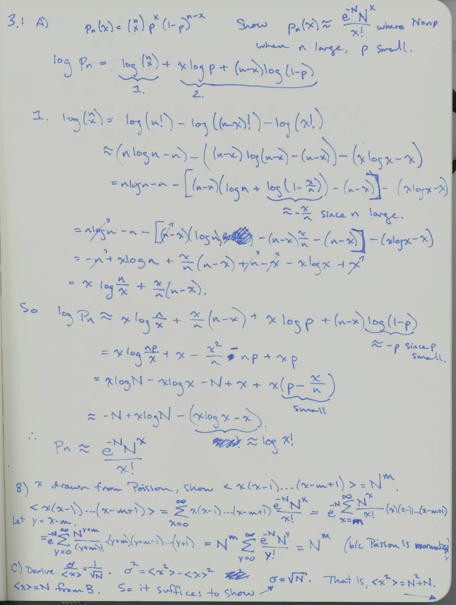
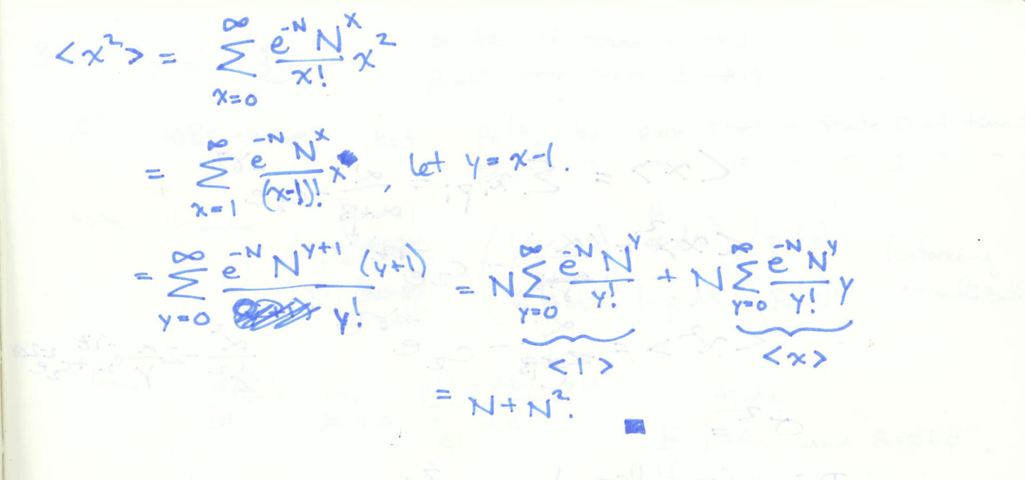
3.1
from scipy.misc import factorial
from scipy.stats import poisson
#def p(x,N):
    #this naive definition will only work for small values on 32-bit install
#    return exp(-N)*(N**x)/factorial(x)
def p(x,N):
    return poisson.pmf(x, N)
t = arange(1,30,dtype=numpy.int64)
for N in [1,4,10,15]:
    plot(t,p(t,N),linestyle='',marker='.',label="N=%d"%N)
legend(loc='upper left')

3.2
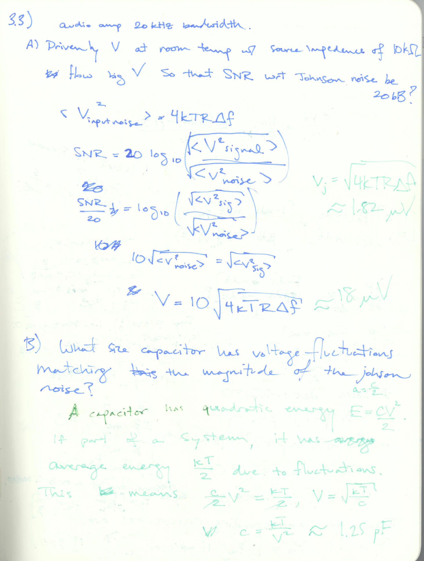
Photons are generated by a light source independently and randomly with an average rate of $N$ per second. How many must be counted by a photodetector per second to determine the rate to within 1%? 1 ppm? What are the corresponding powers in watts for visible light?
Since the photons are random and independent, this is a Poisson process. We saw above that the relative standard deviation is given by $\frac{1}{\sqrt{N}}$, where $N$ is number of events. In our case, this represents detections per second. Thus, to determine the photons per second to within 1%, we must measure $.01^{-2} = 1\times10^{4}$ photons. To within 1 ppm, we must measure $(1\times10^{-6})^{-2} = 1\times10^{12}$.
A photon has energy given by $E = hc/\lambda$, where $\lambda$ is the wavelength. For visible light, say $\lambda = 500 nm$. Then $E = 4.0\times10^{-19} J$ or around $2 eV$.
h = 6.626e-34 #planck const
l = 500e-9 #m, wavelength
c = 3.0e8 #m/s, speed of light
ev = 1.6e-19 #J, electron volt
e_p = h*c/l
print e_p, e_p/ev
def power_print(N):
    print "The wattage of %.0e visible photons per second is %.2e watts."%(N,N*e_p)
power_print(1e4)
power_print(1e12)
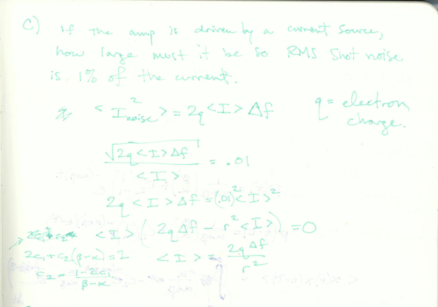
3.3
DF = 20e3 #20 kHz bandwidth
R = 10e3 #10 kOhm source impedance
T = 300 #Kelvin, room temp
snr = 20 #20 db desired snr wrt johnson noise
k = 1.38e-23
def v(df,t,r):
    return 10*sqrt(4*k*t*r*df)
def equiv_cap(v,t):
    #return capacitance in Farads for a capacitor exhibiting fluctuations of voltage v
    return k*t/v/v
figure(figsize=(12,6))
t = linspace(T-50,T+50,100)
r = linspace(R-5e3,R+5e3,100)
df = linspace(DF-9e3,DF+9e3,100)
print "Minimum input voltage: %.2f uV"%(1e6*v(DF,T,R))
print "Johnson noise voltage: %.2f uV"%(1e6*v(DF,T,R)/10)
print "Equivalent capacitance: %.2f nF"%(1e9*equiv_cap(v(DF,T,R)/10,T))
subplot(1, 3, 1)
plot(t,1e6*v(DF,t,R))
xlabel('temperature (K)')
ylabel('required input voltage ($\mu V$)')
grid(True)
subplot(1, 3, 2)
plot(r*1e-3,1e6*v(DF,T,r))
xlabel('resistance ($k\Omega$)')
grid(True)
subplot(1, 3, 3)
plot(df*1e-3,1e6*v(df,T,R))
xlabel('amplifier bandwidth ($kHz$)')
grid(True)

df=20e3 #bandwidth
q = 1.602e-19 #electron charge, Couloumb
def min_current(ratio, df):
    #return minimum current for ratio of current to rms of shot noise to be a given ratio
    #ratio: ratio of shot noise to current
    #df: bandwidth, Hz
    return 2*q*df/ratio/ratio
ratio = .01
print "Current for %.1f%% of rms shot noise to current is %.2e amps"%(100*ratio,min_current(ratio,df))
ri = logspace(-6,0,100)
plot(ri,min_current(ri,df))
gca().set_xscale('log')
gca().set_yscale('log')
xlabel("Ratio rms shot noise to current")
ylabel("Minimum current necessary (amps)")
grid(True)

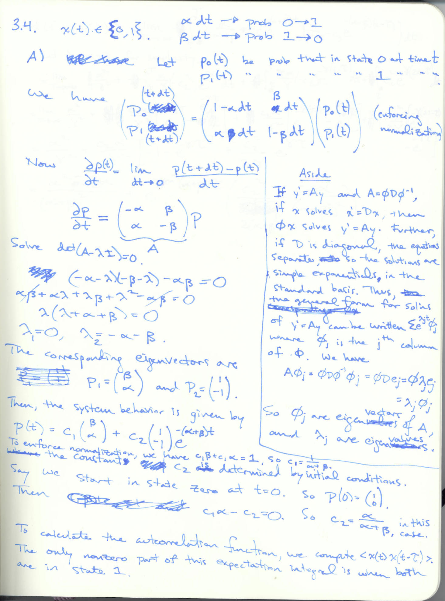
3.4
alpha = .05
beta = .05
gamma = alpha+beta
c1 = 1./gamma
c2 = alpha/gamma
def p(t):
    return asarray(c1*array([beta,alpha]) + c2*exp(-gamma*t[...,None])*array([1,-1]))
def sigma(t):
    mean = alpha/gamma - c2*exp(-gamma*t)
    return sqrt(mean-mean**2)
def R(tau):
    #autocorrelation
    autocovariance = (alpha**2-c2*alpha)/gamma**2 + (c2**2/(2*gamma)+c2*alpha/gamma/gamma)*exp(-gamma*tau)
    return autocovariance#/sigma(tau)
t = linspace(0,20,200)
ax1 = plt.gca()#plt.subplot(211)
ax1.plot(t,p(t)[:,0],label='$p_0$')
ax1.plot(t,p(t)[:,1],label=r'$p_1=\mu$')
#ax1.plot(t,sigma(t),label=r'$\sigma$')
ax1.legend(loc='lower right')
ax1.set_ylim([0,1]);

#ax2 = plt.subplot(212, sharex=ax1)
#ax2.plot(t,R(t),label='$R$',c='r')
#ax2.set_ylim([-1,1])
#ax1.set_title(r'probabilaties, $\alpha=%.2f,\hspace{.5}\beta=%.2f$'%(alpha,beta))
#ax2.set_title('autocorrelation')

For the autocorrelation, we can use these functions to compute the expectation of $\lt x(t) x(t-\tau) \gt$. The expression is only nonzero when both $x(t)$ and $x(t-\tau)$ are nonzero. So, given that $x(t-\tau)$ equals 1, what is probability that $x(t)$ also equals 1? This is exactly the expression we derived above for $p_1$ : $\frac{1}{\alpha+\beta}(\alpha + \beta e^{-(\alpha+\beta)\tau} ) $. This has the right behavior at $\tau=0$ and at steady state.
Since we're taking a limit for the expectation, we can use the steady state probability that the system is in state 1: $\frac{\alpha}{\alpha+\beta}$ as the prior.
Thus, the autocorrelation function is $\lt x(t) x(t-\tau) \gt = \frac{\alpha}{(\alpha+\beta)^2}(\alpha + \beta e^{-(\alpha+\beta)\tau} ) $.
To compute the power spectrum, we need to take a Fourier transform of this autocorrelation (Wiener-Khinchin theroem). Let's just consider a Fourier transform of the form $A+Be^{-\gamma t}$. Fourier is linear, so we can just consider the transorm of a constant and an exponential. The transform of a constant is a delta function. The transform of an exponential can be computed as follows:
$F[e^{-\gamma t}] = \int_0^{\infty} (\cos(2\pi \gamma t) + i \sin(2\pi\gamma t)) e^{-2\pi\gamma t} dt + \int_0^{\infty} (\cos(2\pi \gamma t) - i \sin(2\pi\gamma t)) e^{-2\pi\gamma t} dt$
$F[e^{-\gamma t}] = 2\int_0^{\infty} \cos(2\pi\gamma t)e^{-2\pi\gamma t} dt$
Punting, wolfram says this can be computed by integration by parts:
$F[e^{-\gamma t}](f) = \frac{1}{\pi} \frac{\gamma}{\gamma^2 + f^2}$
Which is a Lorentzian where $\tau = \gamma/2 = \frac{\alpha+\beta}{2}$ in our case.