from numpy import *
%pylab inline
style.use('bmh')

Populating the interactive namespace from numpy and matplotlib

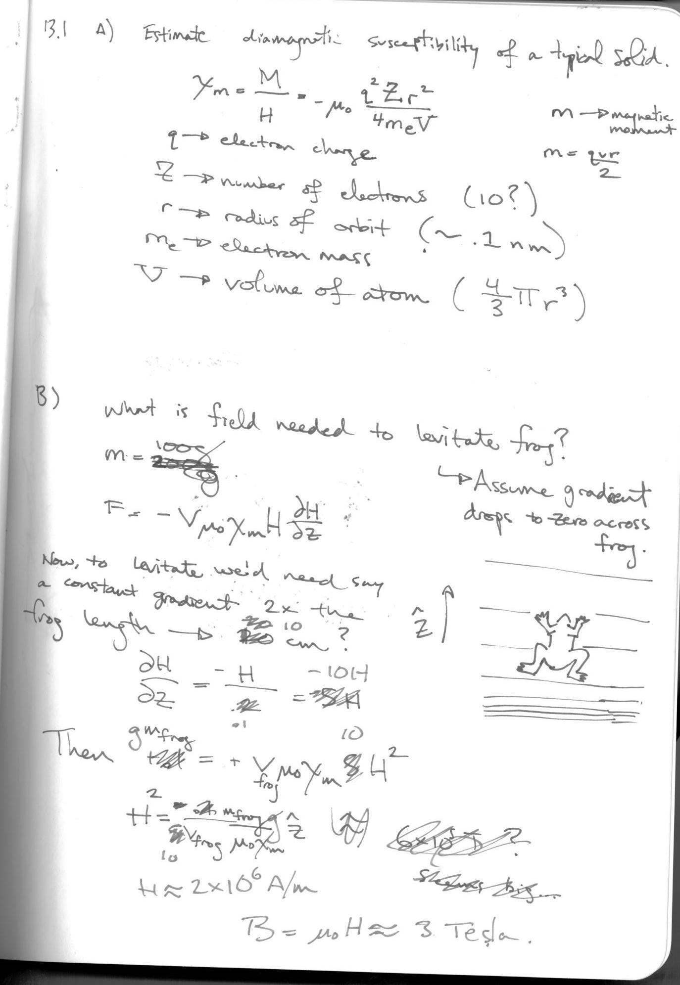
13.1

mu_0 = 4*pi*1e-7
def chi_m(Z,r):
    #estimate of diamagnetic susceptibility
    #Z: number of electrons
    #r: radius of atom
    q = 1.6e-19 #Couloumbs, electron charge
    m = 9.1e-31 #kg, mass of electron
    V = 4/3*pi*r**3
    return -mu_0*(q*q*Z*r*r)/(4*m*V)
Z = 10 #10 electrons
r = .1e-9 #.1 nm atomic radius
chi = chi_m(Z,r)
print "Approximate diamagnetic susceptibility: %.3e, mu_r=%.5f"%(chi, 1+chi)

Approximate diamagnetic susceptibility: -2.813e-04, mu_r=0.99972

r_frog = .05 #meters, radius of frog
v_frog = 4/3*pi*r_frog**3
m_frog = .5 #kg, mass of frog
def H_frog(chi_m, v_frog, m_frog):
    return sqrt( m_frog*9.8 / (10*v_frog*mu_0*chi_m) )
H = H_frog(-chi,v_frog,m_frog)
print "Field to levitate frog: %.2e A/m, %.3f T"%(H,H*mu_0)

Field to levitate frog: 1.88e+06 A/m, 2.361 T

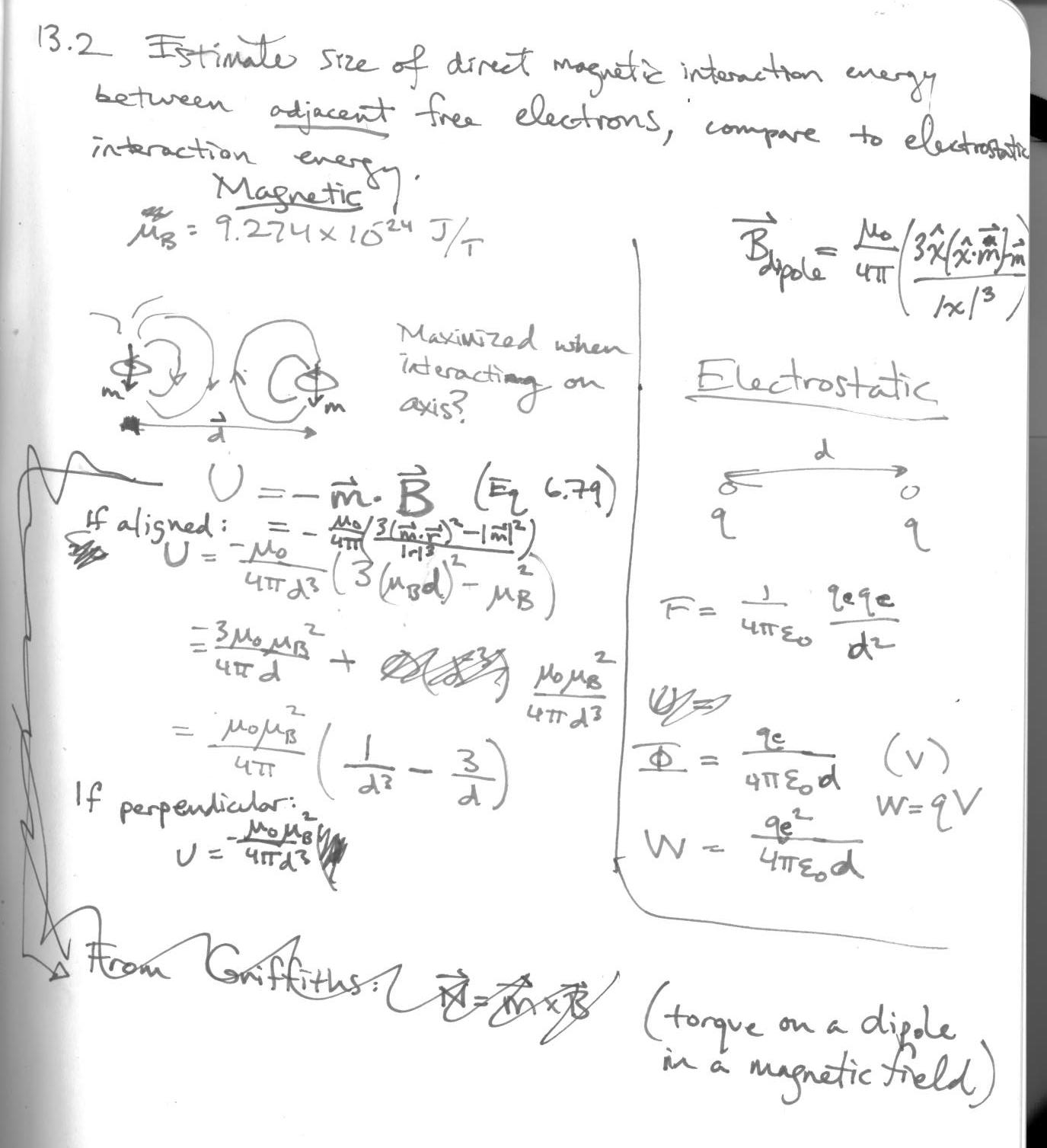
13.2

Estimate size of direct magnetic interaction energy between adjacent free electrons and compare to electrostatic energy.

mu_b = 9.274e-24 #J/T electron spin magnetic moment
eps_0 = 8.85418782e-12
q_e = 1.60217662e-19
def u_mag_aligned(d):
    return mu_0*mu_b**2/4/pi*(1./d**3 - 3./d)
def u_mag_perp(d):
    return mu_0*mu_b**2/4/pi*(1./d**3)
def u_elec(d):
    return q_e**2/4/pi/eps_0/d
d = 1e-10
print "Magnetic interaction energy (aligned): %.2e at %.2e m"%(u_mag_aligned(d),d)
print "Magnetic interaction energy (perpendicular): %.2e at %.2e m"%(u_mag_perp(d),d)
print "Electric interaction energy: %.2e at %.2e m"%(u_elec(d), d)
di = logspace(-14,1,1000)
figure(figsize=(8,6))
plot(di,u_mag_aligned(di), lw=2, label='magnetic interaction energy (aligned)')
plot(di,u_mag_perp(di), lw=2, label='magnetic interaction energy (perpendicular)')
plot(di,u_elec(di), lw=2, label='electric interaction energy')
plot([1e-10,1e-10],[u_mag_aligned(di[0]),u_mag_aligned(di[-1])], color='k',ls='--',label='typical atomic radius')
yscale('log')
xscale('log')
xlabel('separation distance (m)')
ylabel('potential energy (J)')
title('comparing magnetic and electric interaction energies')
legend(loc='lower left')
grid(True)

Magnetic interaction energy (aligned): 8.60e-24 at 1.00e-10 m
Magnetic interaction energy (perpendicular): 8.60e-24 at 1.00e-10 m
Electric interaction energy: 2.31e-18 at 1.00e-10 m

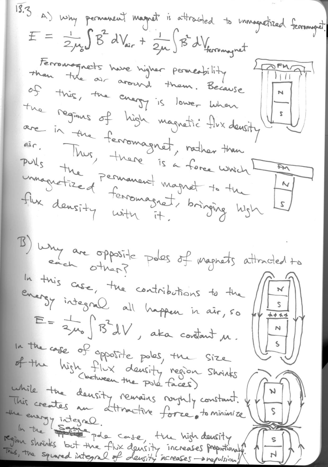
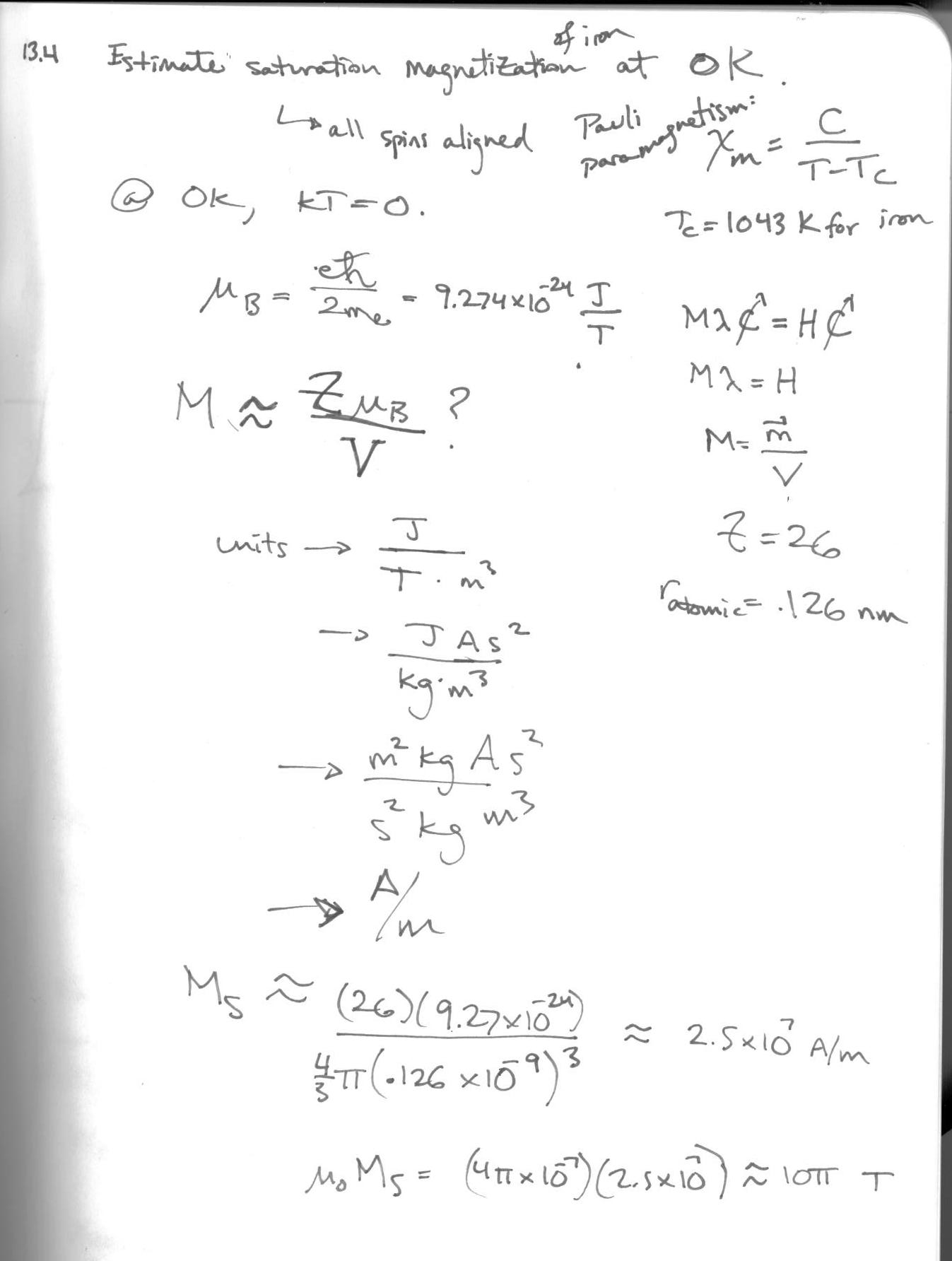
13.3

13.4

Estimate saturation magnetization of iron at 0K.

def m_s(Z,r):
    #approximate magnetic saturation at 0 Kelvin
    #Z: number of electrons
    #r: atomic radius
    mu_b = 9.274e-24 #J/T electron spin magnetic moment
    return Z*mu_b/(4*pi*r**3/3)
print "Approximate saturation magnetism of iron is: %.3e A/m"%(m_s(23,.126e-9))

Approximate saturation magnetism of iron is: 2.546e+07 A/m

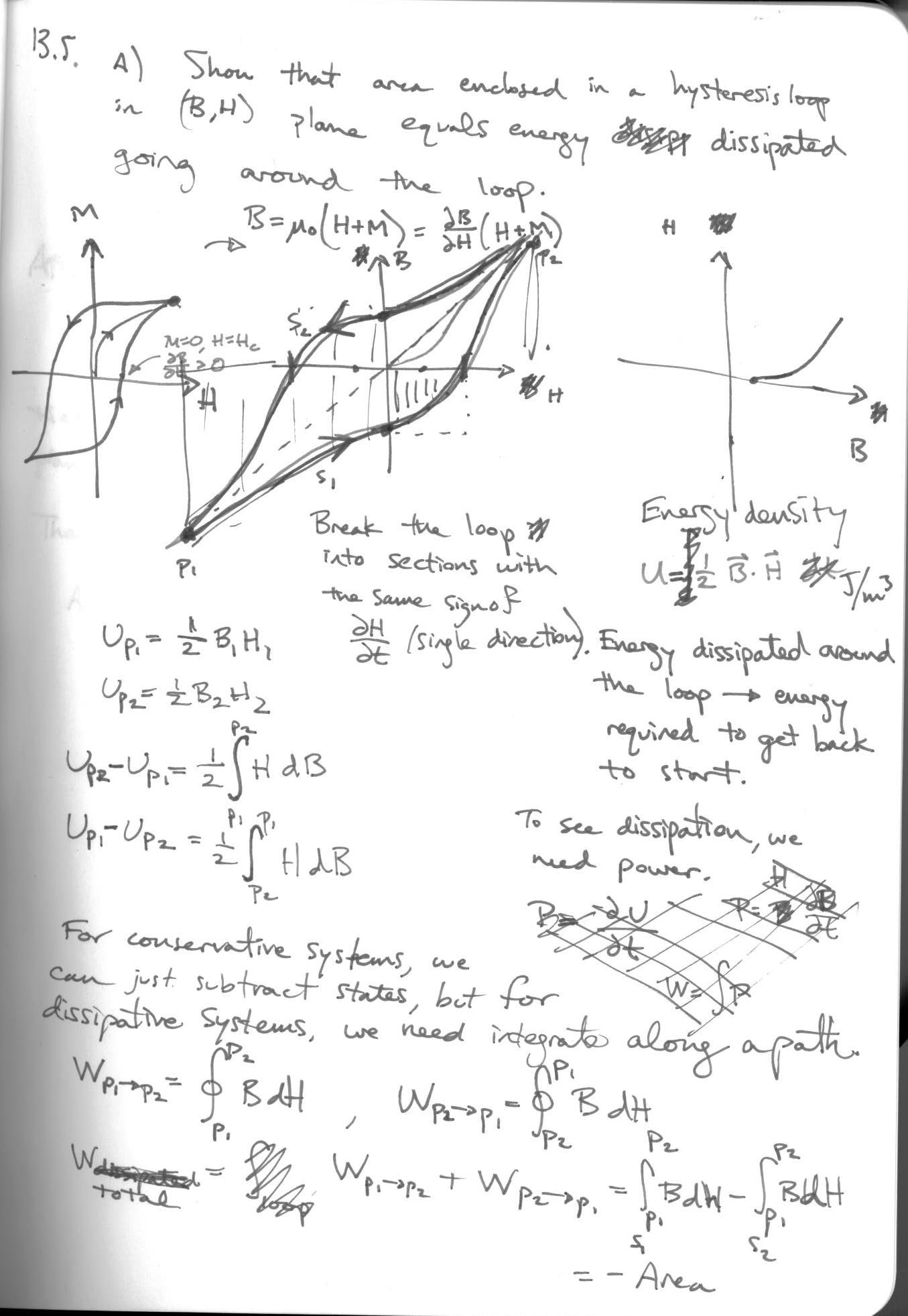
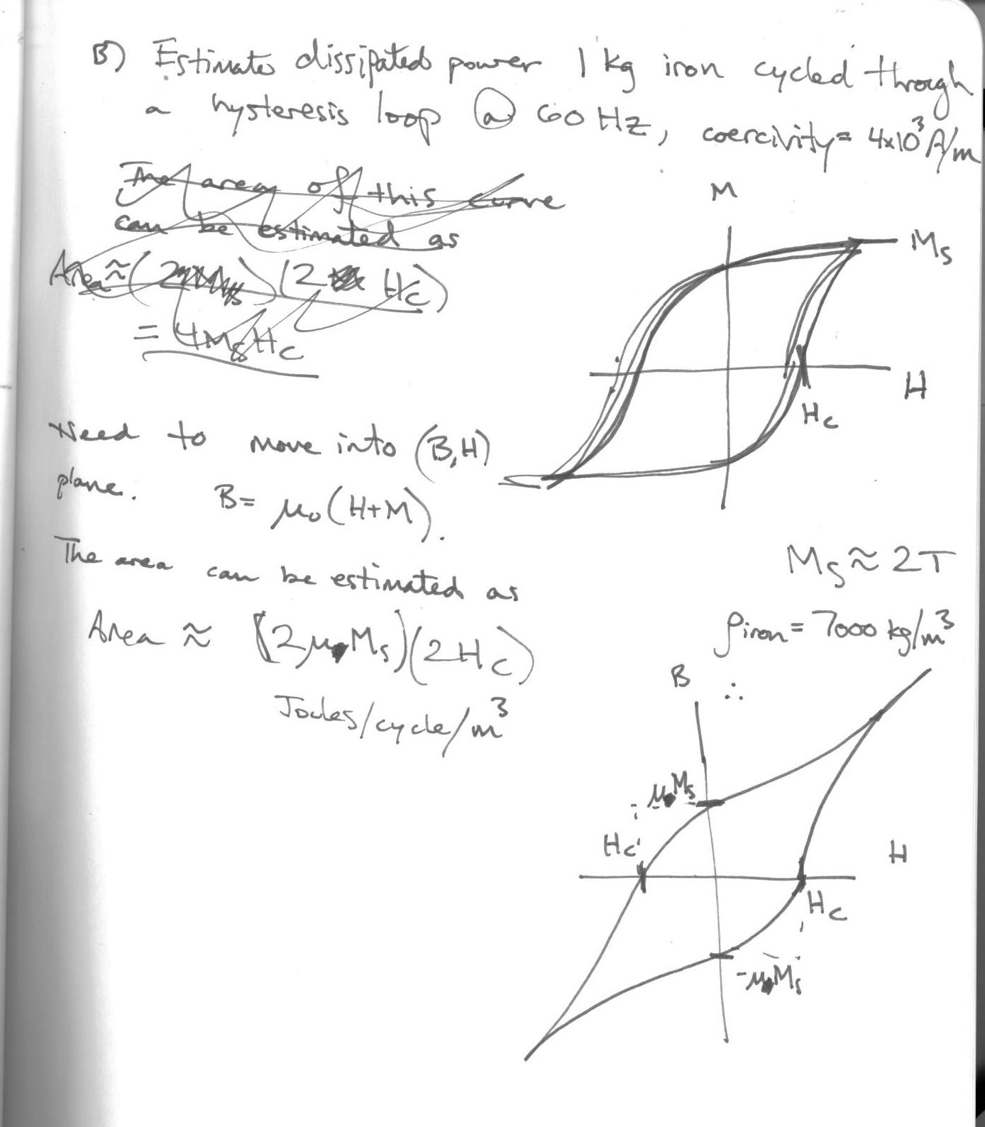
13.5

rho_iron = 7000 #kg/m^3, density of iron
f = 60 #Hz, frequency of cycling
H_c = 4e3 #A/m, coercivity of iron
M_s = 2 #Tesla, saturation magnetism of iron
mu_r = 5000
def cycling_power(f,m):
    #f: frequency
    #m: mass
    V = m/rho_iron
    return f*V*4*mu_0*mu_r*M_s*H_c
m = 1.
print "Power dissipated cycling %.1f kg of iron at %.1f Hz: %.2f Watts"%(m,f,cycling_power(f,m))

Power dissipated cycling 1.0 kg of iron at 60.0 Hz: 1.72 Watts

13.6

<img src='img/p13.6.jpg' width