Problem Set 12

(15.1)

(a)

Show that the circuits in Figures 15.1 and 15.2 differentiate, integrate, sum, and difference.

I’ll take as given that op amps with negative feedback keep their two input terminals at the same voltage. I also assume ideal op-amps that draw no current from their inputs. All the proofs follow from Kirchhoff’s current law (aka conservation of charge). I write $R_f$ to refer to the resistor in the feedback path. All schematics are from Wikimedia Commons.

Integrator

circuit

For the integrator, current through the resistor must equal current through the capacitor.

$\begin{align*} \frac{V_i}{R} &= - C \frac{dV_o}{dt} \\ \frac{dV_o}{dt} &= \frac{-V_i}{R C} \\ V_o &= - \frac{1}{RC} \int V_i \mathrm{d}t \end{align*}$

Differentiator

circuit

For the differentiator, current through the capacitor must equal current through the resistor.

$\begin{align*} C \frac{dV_i}{dt} &= \frac{-V_o}{R} \\ V_o &= -RC \frac{dV_i}{dt} \end{align*}$

Summing Amplifier

circuit

For the summing amplifier, the sum of the currents through the input resistors must equal the current through the feedback resistor.

$\begin{align*} \frac{V_1 + \cdots + V_n}{R_i} &= -\frac{V_o}{R_f} \\ V_o &= -\frac{R_f}{R_i} (V_1 + \cdots + V_n) \end{align*}$

Differential Amplifier

circuit

For the difference amplifier, neither input terminal is grounded, so we can’t assume they’re at zero volts. Call their voltage $V_i$ . I’ll also assume both resistors $R_1$ and $R_2$ in the above schematic are the same, which I’ll call $R_i$ . Applying Kirchhoff’s current law to the non-inverting input,

$\begin{align*} \frac{V_2 - V_i}{R_i} &= \frac{V_i}{R_f} \\ \frac{V_2}{R_i} &= V_i \left( \frac{1}{R_i} + \frac{1}{R_f} \right) \end{align*}$

Then looking at the inverting input,

$\begin{align*} \frac{V_1 - V_i}{R_i} &= \frac{V_i - V_o}{R_f} \\ \frac{V_1}{R_i} - \frac{V_o}{R_f} &= V_i \left( \frac{1}{R_i} + \frac{1}{R_f} \right) \\ \frac{V_1}{R_i} - \frac{V_o}{R_f} &= \frac{V_2}{R_i} \\ V_o &= \frac{R_f}{R_i} (V_2 - V_1) \end{align*}$

(b)

Design a non-inverting op-amp amplifier. Why are they used less commonly than inverting ones?

circuit

Connect the signal you want to amplify to the non-inverting input. Then create a voltage divider, connected to ground on one end, the inverting input in the middle, and the output on the other end. I’ll call the resistor connected to ground $R_g$ , and the feedback resistor $R_f$ as before.

$\begin{align*} \frac{V_o - V_i}{R_f} &= \frac{V_i}{R_g} \\ \frac{V_o}{R_f} &= V_i \frac{R_f + R_g}{R_f R_g} \\ V_o &= V_i \left( 1 + \frac{R_f}{R_g} \right) \end{align*}$

A potential downside is that the gain must be at least unity. Additionally the nodes aren’t tied to ground, so if the op-amp has imperfect common-mode rejection we’ll see it in the output. A potential upside is that the input impedance is very high. And, of course, the output isn’t inverted.

(c)

Design a transimpedance (voltage out proportional to current in) and a transconductance (current out proportional to voltage in) op-amp circuit.

circuit

For a transimpedance amplifier, replace the input resistor in an inverting amplifier with a wire. Then the current flowing through the feedback resistor is equal to the current at the input. So $I = V_o / R_f$ , and $V_o = R_f I$ .

For a transconductance amplifier, replace the feedback resistor with a wire. Then the current out is $I = -V_i / R_i$ . If you want a non-inverting transconductance amplifier, connect the input straight to the non-inverting terminal and connect the inverting terminal to ground via a resistor $R_g$ . Then $I = V_i / R_g$ .

(d)

Derive equation (15.16).

The currents flowing through $R_1$ , $R_o$ , and $C$ must be equal. Call this current $I$ (I’ll take left to right to be positive for all currents). Because of the negative feedback, the inverting input of the op-amp is a virtual ground. Recall that $Q = CV$ , so $dQ/dt = I = C dV/dt$ . Thus we can express $I$ three ways:

$\begin{align*} I &= \frac{V_{PD}}{R_1} \\ &= -\frac{V_{RC}}{R_0} \\ &= C \left( \frac{dV_{RC}}{dt} - \frac{dV_F}{dt} \right) \end{align*}$

I’m using $V_{RC}$ to denote the voltage at the junction between $R_O$ and $C$ . Differentiating the first two lines yields

$\begin{align*} \frac{dI}{dt} &= \frac{1}{R_1} \frac{dV_{PD}}{dt} \\ &= -\frac{1}{R_0} \frac{dV_{RC}}{dt} \end{align*}$

Thus

$\frac{dV_{RC}}{dt} = -\frac{R_0}{R_1} \frac{dV_{PD}}{dt}$

As such we can write the current through the capacitor as

$I = C \left( -\frac{R_0}{R_1} \frac{dV_{PD}}{dt} - \frac{dV_F}{dt} \right)$

This can still be equated

$C \left( -\frac{R_0}{R_1} \frac{dV_{PD}}{dt} - \frac{dV_F}{dt} \right) = \frac{V_{PD}}{R_1}$

So all that remains is to solve for $dV_F/dt$ .

$\frac{dV_F}{dt} = \frac{V_{PD}}{R_1 C} + \frac{R_0}{R_1} \frac{dV_{PD}}{dt}$

This differs in sign from (15.16) because the book makes the positive current direction right to left.

(15.2)

If an op-amp with a gain–bandwidth product of 10 MHz and an open-loop DC gain of 100 dB is configured as an inverting amplifier, plot the magnitude and phase of the gain as a function of frequency as $R_\text{out}/R_\text{in}$ is varied.

(15.3)

A lock-in has an oscillator frequency of 100 kHz, a bandpass filter Q of 50 (re- member that the Q or quality factor is the ratio of the center frequency to the width between the frequencies at which the power is reduced by a factor of 2), an input detector that has a flat response up to 1 MHz, and an output filter time constant of 1 s. For simplicity, assume that both filters are flat in their passbands and have sharp cutoffs. Estimate the amount of noise reduction at each stage for a signal corrupted by additive uncorrelated white noise.

(15.4)

(a)

For an order 4 maximal LFSR work out the bit sequence.

Table (13.1) indicates that a maximal LFSR of order 4 is $x_n = x_{n-1} + x_{n-4}$ . The bit sequence has to repeat in a cycle of length $2^4 - 1 = 15$ . The bits are 1, 1, 1, 1, 0, 1, 0, 1, 1, 0, 0, 1, 0, 0, 0.

(b)

If an LFSR has a chip rate of 1GHz, how long must it be for the time between repeats to be the age of the universe?

The age of the universe is 13.7 billion years, which is about $\num{43e16}$ seconds.

$\begin{align*} (2^N - 1) \cdot 10^{-9} \si{s} = \num{43e16} \si{s} \\ (2^N - 1) = \num{43e25} N = 88.5 \end{align*}$

(c)

Assuming a flat noise power spectrum, what is the coding gain if the entire sequence is used to send one bit?

I think the coding gain works out like the SNR I derive in the next problem… but could be wrong.

$10 \log_{10} \left( 2^{88.5} \right) = 266 \si{dB}$

(15.5)

What is the SNR due to quantization noise in an 8-bit A/D? 16-bit? How much must the former be averaged to match the latter?

This depends on the characteristics of the signal. Assuming that it uses the full range of the A/D converter (but no more), and over time is equally likely to be any voltage in that range, then the SNR in decibels is

$\text{SNR} = 20 \log_{10}(2^n)$

where $n$ is the number of bits used.

So we have

$\begin{align*} \text{8-bit SNR} &= 20 \log_{10}(2^8) \\ &= 48.2 \si{dB} \\ \text{16-bit SNR} &= 20 \log_{10}(2^{16}) \\ &= 96.3 \si{dB} \end{align*}$

But where does this come from? Recall that the definition of the SNR is the ratio of the power in the signal to the power in the noise. Let’s say we have an analog signal $f(t)$ within the range $[-A, A]$ . Let its time-averaged distribution be $p(x)$ . Then the power in the signal is

$P_\text{signal} = \int_{-A}^A x^2 p(x) \mathrm{d} x$

Let’s assume that the signal is equally likely to take on any value in its range, so $p(x) = 1/(2A)$ . This is completely true of triangle waves and sawtooth waves, relatively true for sin waves, but not true at all for square waves. So this approximation may or may not be very accurate. Then its power is

$\begin{align*} P_\text{signal} &= \frac{1}{2A} \int_{-A}^A x^2 \mathrm{d} x \\ &= \frac{1}{2A} \frac{1}{3} \left[ x^3 \right]_ {-A}^A \\ &= \frac{1}{2A} \frac{1}{3} 2A^3 \\ &= \frac{A^2}{3} \end{align*}$

When the signal is quantized, each measurement $f(t)$ is replaced with a quantized version. The most significant bit tells us which half of the signal range we’re in. In this case that means whether we’re in the range [-A, 0] or [0, A]. Note that each interval is $A$ long. The next bit tells us which half of that half we’re in. Each interval is $A/2$ long. So finally the least significant bit will tell us which half of a half etc. we’re in, and each interval will be $A/2^{n - 1}$ long (or equivalently $2A/2^n$ ), where $n$ is the number of bits.

The uncertainty we have about the original value is thus plus or minus half the least significant bit. So the quantization error will be in the range $[-A/2^n, A/2^n]$ . Since we’re assuming our signal is equally likely to take any value, the quantization error is equally likely to fall anywhere in this range. Thus the power in the quantization noise is

$\begin{align*} P_\text{noise} &= \frac{2^n}{2A} \int_{-A/2^n}^{A/2^n} x^2 \mathrm{d} x \\ &= \frac{2^n}{2A} \frac{1}{3} \left[ x^3 \right]_ {-A/2^n}^{A/2^n} \\ &= \frac{2^n}{2A} \frac{1}{3} \frac{2 A^3}{2^{3n}} \\ &= \frac{A^2}{3} \frac{1}{2^{2n}} \end{align*}$

Putting it together,

$\begin{align*} \text{SNR} &= 10 \log_{10} \left( \frac{P_\text{signal}}{P_\text{noise}} \right) \\ &= 10 \log_{10} \left( \frac{A^2}{3} \cdot \frac{3}{A^2} \frac{2^{2n}}{1} \right) \\ &= 10 \log_{10} \left( 2^{2n} \right) \\ &= 20 \log_{10} \left( 2^n \right) \end{align*}$

(15.6)

The message 00 10 01 11 00 ( $c_1$ , $c_2$ ) was received from a noisy channel. If it was sent by the convolutional encoder in Figure 15.20, what data were transmitted?

(15.7)

This problem is harder than the others.

My code for all sections of this problem is here. All the sampling and gradient descent is done in C++ using Eigen for vector and matrix operations. I use Python and matplotlib to generate the plots.

(a)

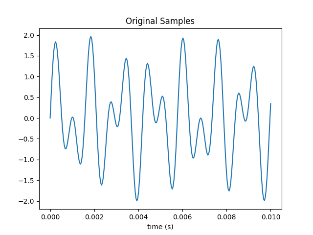
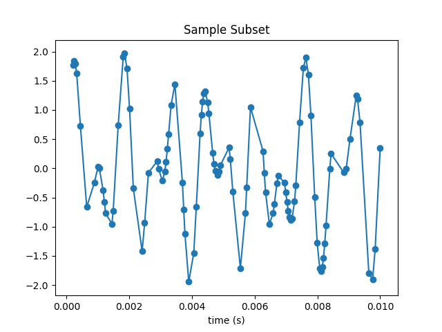
Generate and plot a periodically sampled time series { $t_j$ } of N points for the sum of two sine waves at 697 and 1209 Hz, which is the DTMF tone for the number 1 key.

Here’s a plot of 250 samples taken over one tenth of a second.

samples

(b)

Calculate and plot the Discrete Cosine Transform (DCT) coefficients { $f_i$ } for these data, defined by their multiplication by the matrix $f_i = \sum_{j = 0}^{N - 1} D_{ij} t_j$ , where

$\begin{align*} D_{ij} = \begin{cases} \sqrt{\frac{1}{N}} &(i = 0)\\ \sqrt{\frac{2}{N}} \cos \left( \frac{\pi (2j + 1) i}{2 N} \right) &(1 \leq i \leq N - 1) \end{cases} \end{align*}$

dct

(c)

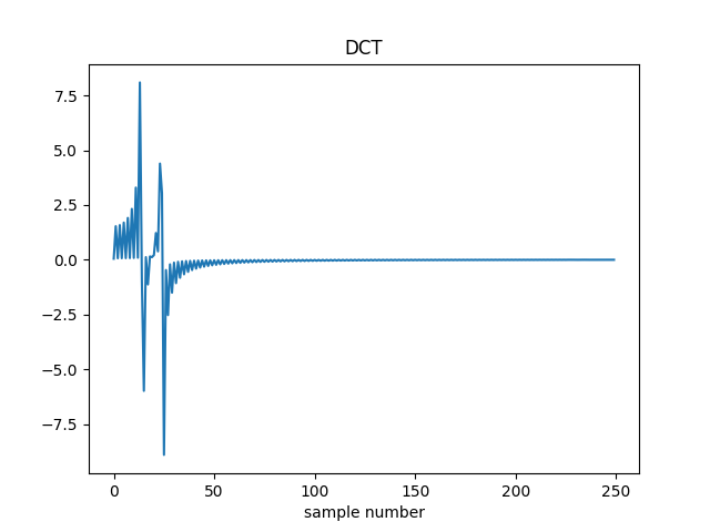
Plot the inverse transform of the { $f_i$ } by multiplying them by the inverse of the DCT matrix (which is equal to its transpose) and verify that it matches the time series.

The original samples are recovered.

recovered samples

(d)

Randomly sample and plot a subset of M points { $t^\prime_k$ } of the { $t_j$ }; you’ll later investigate the dependence on the sample size.

Here I’ve selected 100 samples from the original 250. The plot is recognizable but very distorted.

subset samples

(e)

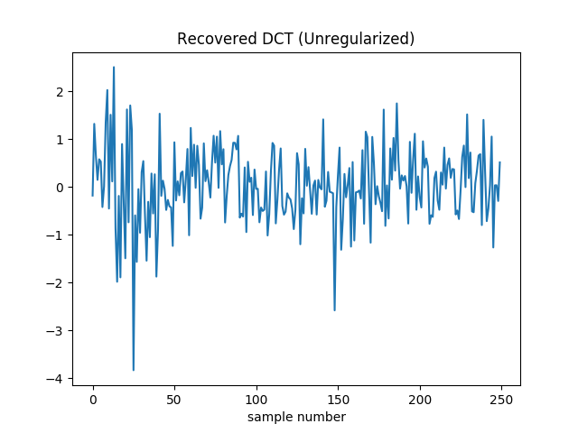
Starting with a random guess for the DCT coefficients { $f^\prime_i$ }, use gradient descent to minimize the error at the sample points

$\min_{\{f^\prime_i\}} \sum_{k = 0}^{M - 1} \left( t^\prime_k - \sum_{j = 0}^{N - 1} D_{ij} f^\prime_i \right)^2$

and plot the resulting estimated coefficients.

Gradient descent very quickly drives the loss function to zero. However it’s not reconstructing the true DCT coefficients.

recovered dct (unregularized)

To make sure I don’t have a bug in my code, I plotted the samples we get by performing the inverse DCT on the estimated coefficients.

recovered samples (unregularized)

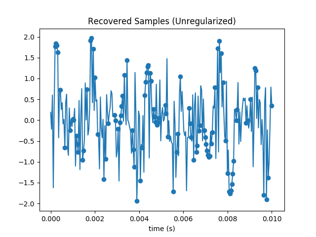
Sure enough all samples in the subset are matched exactly. But the others are way off the mark. We’ve added a lot of high frequency content, and are obviously overfitting.

(f)

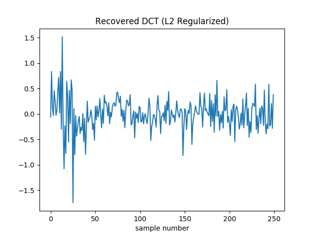
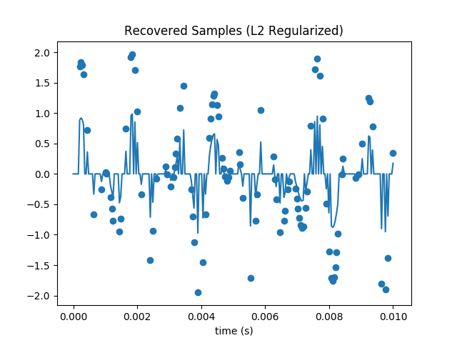
The preceding minimization is under-constrained; it becomes well-posed if a norm of the DCT coefficients is minimized subject to a constraint of agreeing with the sampled points. One of the simplest (but not best [Gershenfeld, 1999]) ways to do this is by adding a penalty term to the minimization. Repeat the gradient descent minimization using the L2 norm:

$\min_{\{f^\prime_i\}} \sum_{k = 0}^{M - 1} \left( t^\prime_k - \sum_{j = 0}^{N - 1} D_{ij} f^\prime_i \right)^2 + \sum_{i = 0}^{N - 1} f^{\prime 2}_i$

and plot the resulting estimated coefficients.

With L2 regularization, we remove some of the high frequency content. This makes the real peaks a little more prominent.

recovered dct (L2 regularized)

However it comes at a cost: gradient descent no longer drive the loss to zero. As such the loss itself isn’t a good termination condition. In its place I terminate when the squared norm of the gradient is less than $\num{1e-6}$ . The final loss for the coefficients in the plot above is around 50.

You can easily see that the loss is nonzero from the reconstructed samples.

recovered samples (L2 regularized)

(g)

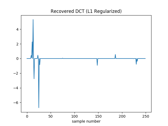
Repeat the gradient descent minimization using the L1 norm:

$\min_{\{f^\prime_i\}} \sum_{k = 0}^{M - 1} \left( t^\prime_k - \sum_{j = 0}^{N - 1} D_{ij} f^\prime_i \right)^2 + \sum_{i = 0}^{N - 1} \vert f^{\prime}_i \vert$

Plot the resulting estimated coefficients, compare to the L2 norm estimate, and compare the dependence of the results on M to the Nyquist sampling limit of twice the highest frequency.

With L1 regularization the DCT coefficients are recovered pretty well. There is no added high frequency noise.

recovered dct (L1 regularized)

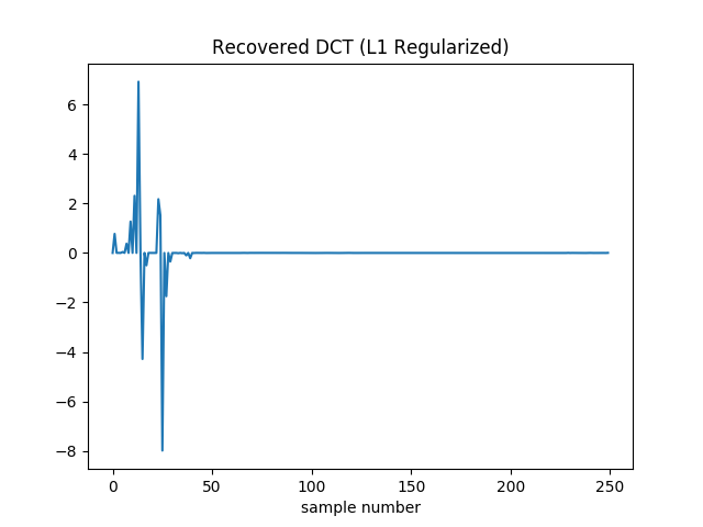
It still can’t drive the loss to zero. Additionally it’s hard to drive the squared norm of the gradient to zero, since the gradient of the absolute values shows up as 1 or -1. (Though to help prevent oscillation I actually drop this contribution if the absolute value of the coefficient in question is less than $\num{1e-3}$ .) So here I terminate when the relative change in the loss falls below $\num{1e-9}$ . I also decay the learning rate during optimization. It starts at 0.1 and is multiplied by 0.99 every 64 iterations.

The final loss is around 40, so better than we found with L2 regularization. However it did take longer to converge: this version stopped after 21,060 iterations, as opposed to 44 (for L2) or 42 (for unregularized). If I stop it after 50 samples it’s a bit worse than the L2 version (loss of 55 instead of 50). It’s not until roughly 2500 iterations that it’s unequivocally pulled ahead. I played with learning rates and decay schedules a bit, but there might be more room for improvement.

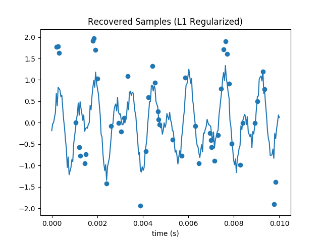
The recovered samples are also much more visually recognizable. The amplitude of our waveform seems overall a bit diminished, but unlike our previous attempts it looks similar to the original.

recovered samples (L1 regularized)

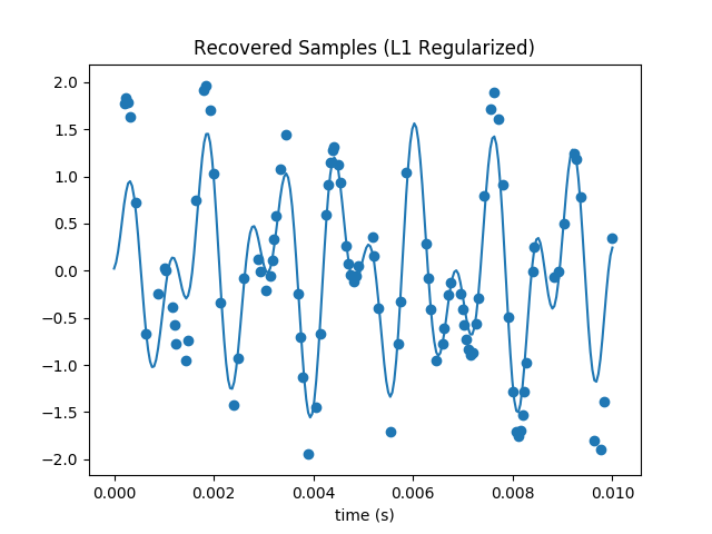
This technique can recover the signal substantially below the Nyquist limit. The highest frequency signal is 1209 Hz, so with traditional techniques we’d have to sample at 2418 Hz or faster to avoid artifacts. Since I’m only plotting over one hundreth of a second, I thus need at least 242 samples. So my original 250 is (not coicidentally) near here. But even with a subset of only 50 samples, the L1 regularized gradient descent does an admirable job at recovering the DCT coefficients and samples:

recovered dct (from 50) recovered samples (from 50)