![]()
![]()
- 1. project description
1.1. Project description:
This week I made different four different sensors: a light sensor, two step response sensors (load and txrx) and a sound sensor. For the light and step response I implemented Neil's design. For the sound sensor, I decided to reverse engineer Neil's board and design it in the Eagle PCB Software. This was very good practice as it gave me the opportunity to start a schematic from scratch in Eagle knowing the components and the way they are connected. From the schematic I then moved to route the traces on the board trying to use different arrangements than the initial design. I will go through each one of the sensors documenting their operation with videos and photos, as well as describing particularities about the process of making and programming it where necessary.
Figure 1: The boards that I made this week; right to left are the "txrx" step response sensor, the "load" step response sensor, the light sensor with the phototransistor and the sound sensor with the electret microphone
1.2. Light sensor:
I made this board using Neil's design. The milling and soldering were completed without any problems. When it came to the programming of the board I kept getting an error when I was trying to open a serial port. This was probably due to the fact that I had two versions of python on my computer (2.6.1 and 2.7). I removed version 2.7 and the problem was resolved.These are the steps that I followed for programming.
cd /Users/TheodoraVardouli/Desktop/light // find the directory
make -f hello.light.45.make // compile the program
make -f hello.light.45.make program-usbtiny // write program on board using FabISP in circuit programmer
python hello.txrx.45.py // run the python code
python hello.txrx.45.py /dev/tty.usbserial-FTF61DID // open a serial port (it is assigned automatically by pressing auto-complete [Tab] after typing usbserial-)As shown in the video below, the sensor gives higher values when someone goes closer to the phototransistor.

Figure 2: The light sensor board
Figure 3: video of the light sensor operation
1.3. Step response sensor - Load:
After having designed the light sensor I did the step response sensors starting from the load board, again provided by Neil.

Figure 4: The "Load" step response sensor board
I milled and stuffed the board, programmed it, but when I tried to open the serial port the application kept freezing. The reason for that was that the board did not give the correct readings and was stuck in an infinite loop from which it never broke. This is the part of Neil's python code that dictated that:
from hello.load.45.py:
while 1:
byte1 = byte2
byte2 = byte3
byte3 = byte4
byte4 = ord(ser.read())
if ((byte1 == 1) & (byte2 == 2) & (byte3 == 3) & (byte4 == 4)):
breakMoritz helped me intercept the sensor readings through Serial Tools, which confirmed that the sensor never read the 1,2,3,4 pattern.
In the beginning I thought that there was something wrong with the board but Shahar pointed out that the problem might be a timing error. I changed the bit delay for 9600 from 100 to 101 in the .c code and it worked! I reprogrammed the board and connected it to a copper plate through a piece of wire. I was getting slighlty confused about which pin I should connect to the copper plate so I tried all of them consecutively and only kept the one that was giving me a measurement.
Figure 5: video of the "Load" step response sensor operation
1.4. Step response sensor - TXRX:
The TXRX sensor measures the capacitance between two different copper plates. The design is again based on Neil's transmit-receive board. I used the same technique as with the load sensor (testing all of them) to identify which two pins should be connected to the copper plates.

Figure 5: The "transmit-receive" step response sensor connected to the copper plates
The initial reading that I was geting was very low, as shown in the first video below. Also, a comment which is also valid for the load sensor, the measurement changed only when one touched the copper plates and not when one approached them. In order to make the sensor more sensitive, I modified Neil's python code so that instead of mapping the sensor values into the graph using 10000 as a divider it now uses 1000. This is more sensitive than the sensor should be and perhaps calls for a divider value for abput 2000.
from hello.txrx.45.py:
value = (up_value - down_value)
filt = (1-eps)*filt + eps*value
x = int(.2*WINDOW + (.9-.2)*WINDOW*filt/1000.0)
Figure 6: TXRX weak reponse to touch
Figure 7: TXRX after changing the python code; the sensitivity of the sensor has signifantly increased
1.5. Sound:
That was the last but most challenging part of the assignment. Not having any prior experience in designing boards from scratch I decided that trying to do that for the sound sensor would be an educational experience.

Figure 6: The sound sensor
I used the Eagle PCB Software to reverse engineer and redesign Neil's electret microphone board.
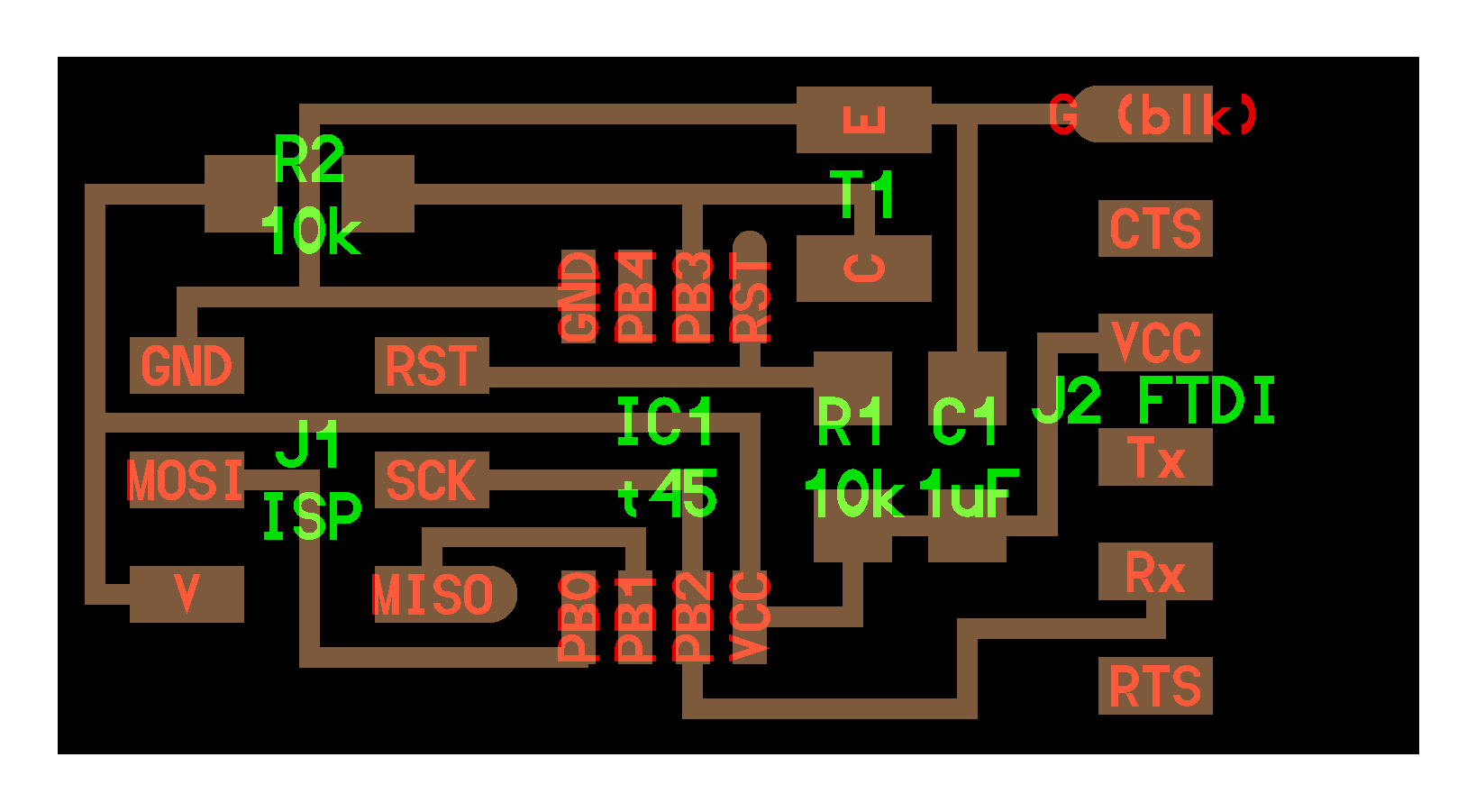
Figure 9: Schematic in Eagle PCB software, based on the connections of the given sound sensor board
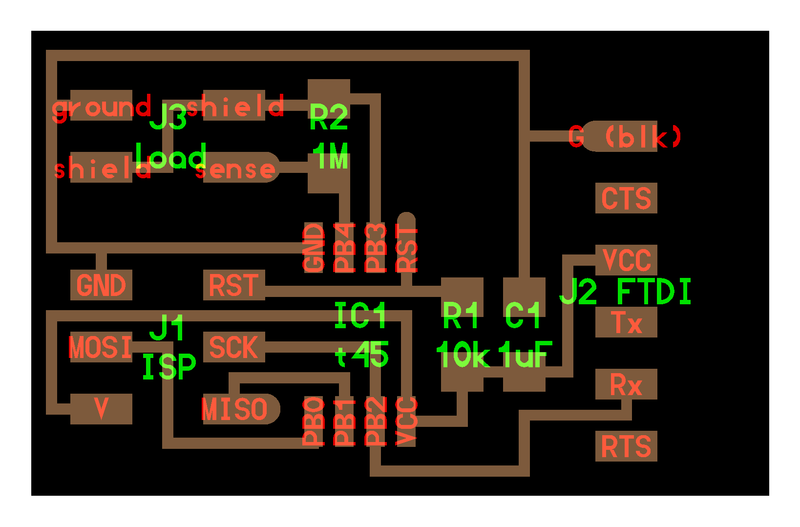
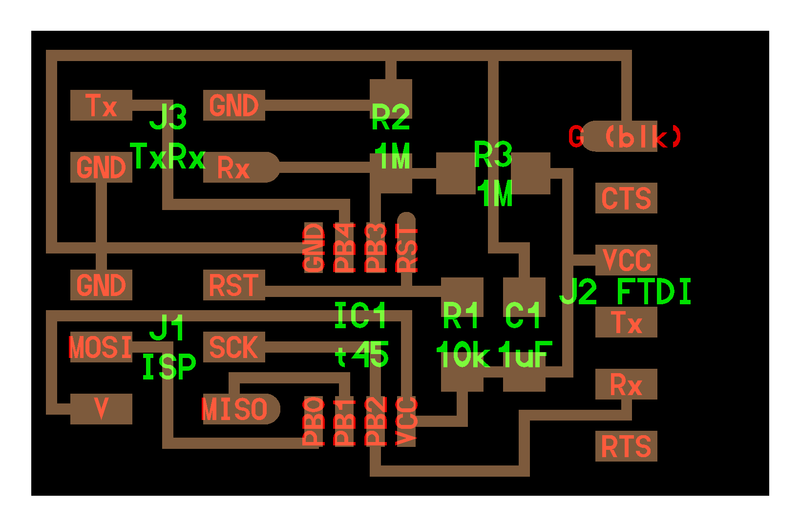
After the schematic, I routed the connections in Eagle. I did not manage to recreate all the necessary connections in the schematic, so I had to do some of them manually after exporting the .png image of the traces from Eagle. During this process of postprocessing in Adobe Photoshop I also manually increased the distance between some of the traces.

Figure 10: The traces of the sound sensor based on the schematic I recreated in Eagle

Figure 11: Fab modules for Roland Modela

Figure 12: Milling the board on the Roland Modela
I milled and stuffed the board but when I tried to program it it constantly gave me an rc-1 error reading:
avrdude: initialization failed, rc=-1
Double check connections and try again, or use -F to override
this check..I checked the board multiple times and after a quite a bit of debugging, I decided to look back at the Eagle file. I realized that one of the connections which was under the microcontroller was left unrouted (Tip: always run ratsnest even if you are confident you got everything. I had to connect the RESET pin with the 10K Resistor with exra solder to make up for the missing trace. After doing that I got the board to program but all I was getting was noise. I suspect that one of the components is not soldered correctly.

Figure 13: The board is programmed but it only outputs noise
I realized that the problem was that I had connected the 0.1uF and 1uF capacitors in the wrong positions and they had to be reversed. However, I decided to remill the board so that I get the traces and the components correct from the beginning. This time it worked! Here is the sound sensor listening to the Beatles.
Figure 14: I remilled and restuffed the board and it finally worked!

2.1. Tutorial at the CBA:
On Tuesday morning John Difrancesco and Tom Lutz showed us how to use the Konica Minolta 3D Digitizer, with the Geomagic software. I brought a wooden mannequin for testing. We decided to scan only its legs for demonstration. The result was very good besides the initial anxiety about the model moving while the table was rotating during the multi-shot scan. Tom also showed us the NextEngine 3d Laser Scanner, which he used to scan a matchbox. Compared to the Minolta, the scanner is slower with relatively worse software support (ScanStudio HD). Below are some snapshots from the tutorial.


Figure 9: Left - testing the Konica Minolta Digitizer with a mannequin; Right - testing the Next Engine 3d Laser Scanner with a matchbox
2.2. Artist's mannequin with Hand Held Z-Corp 3d Scanner:
After having tried the mannequin at the Konica Minolta with John, I decided to use the Architecture Shop Hand Held Z-Corp 3d Scanner, which comes with the ZScan 3d Digitizing Software. The Scanner requires the following steps:
1. sensor calibration with an image that comes with the scanner package
2. sensor configuration with the object which is being scanned
3. positioning features scanning; these are the white stickers that you see in the image below. They are used to create a coordinate system for the scanner in relation to the geometry of the object
4. object scanning

Figure 10: The mannequin covered with stickers which operate as positioining features

Figure 10: Snapshots from the ZScan Environment - Left: scanning the positioning features; Right: Scanning the object

Figure 11: The .stl model from the mannequin scan with the ZCorp hand-held 3d scanner
I tried two times but the result that I got was not satisfactory for the entire figure. Some parts of it were scanner smoothly and accurately but other parts were left open although I persistently tried to fill them in while scanning. One problem was the metal rod that was holding the mannequin which was occasionally shooting off reflections causing noise in the scan.
2.3. Artist's mannequin with Konica Minolta Digitizer (take 2):
In my second attempt at the Konica Minolta, the attachement of the mannequin to the vertical metal rod had become even looser, causing the object to move while the plate was rotating. Although the indvidual scans were very good, the stiching between them became very problematic.
Figure 12: An .stl model from the Konica Minolta Digitizer; the motion of the model during the scanning caused problems in the stitching of the pieces
2.4. Artist's mannequin with Konica Minolta Digitizer (take 3):
This time I made sure to change the position of the mannequin so that it is more stable and to put some hot glue at the point where the supporting metal rod meets the mannequin. The result was much better.
Figure 13: The .stl model from the mannequin scan with the Konica Minolta Digitizer
1.5. Russian Doll with Konica Minolta:
After having scanned the mannequin I scanned a Russian Doll thatn I have had since I can remember myself. I used 90 degrees multishot scan, which came out good. I used geomagic to patch some minor holes.
Figure 14: Scanning and using the Geomagic Software at the CBA shop
Figure 15: The .stl model from the russian doll scan with the Konica Minolta Digitizer
On Wednesday morning John and Tom gave us a tutorial on how to use the laser cutter. Here is a transcript of the notes that I kept along with some tips from personal experience.
3.1. Safety first:
It is quite usual to see a small flame when the laser is cutting the material. If a small flame worries you then you can open the lid and cover the flame with a piece of acrylic. If the flame is big or the material catches on fire then you open the lid, close the air valve and call 100.3.2. How to put the material on the laser bed:
The origin point is the top left corner. Make sure your material is the right size; in the Universal Laser Cutter at the CBA shop the bed is 32*18". You might need to use some tape to attach the material to the edges of the bed if it is not completely flat (this is for example very usual with cardboard)3.3. How to adjust the height of the laser bed:
Use the marked metal rod to measure the height between the cutting tool and the material you have placed on the laser cutter board. Press Z and use the Up and Down arrows to bring the cutting material to the edge of the metal rod. You will know that the height is right when the pin does not let the board to go any further up.
The check button moves to smaller digit precision for height refinements with the up and down arrows. Once you have found the right height press Z again to exit.3.4. How to send your files:
3.4.1. If you are using Inkscape:
1. Prepare your file and export it in 300dpi. Keep in mind that the white part is the one cut with precision so your offsets are "eating" off the black part.
2. Go to fab > run in terminal
3. Select the Universal laser cutter and define power and speed. Make sure that you set the pulses per inch (ppi) to be less than 500 if you are cutting cardboard. If you are cutting acrylic you can do almost 300.
4. Specify xmin and ymin. This is how far from the top left corner (origin) the machine will start cutting the file.
Hit make .uni
6. Send!3.4.2. If you are using CorelDraw (Windows):
1. Import your file
2. Make sure all your lines are Hairline (No thickness)
3. Optional step: You might want to offset your lines for precision. Go to Effects>Contour and do an Outside offset of 0.005 (or around that) Then do Arrange and break contour group apart.
4. Go to File>Print>Properties and set Power and Speed per color
Press Set to register your changes
6. Print!3.4.3. If you are using Rhino or AutoCAD (Windows) you can set the speed and power per layer through the print menu. Make sure you SKIP all the layers you do not want to cut and that you select the area you want to cut with a print window and that all your lines are 0 thickness or hairlines. In Rhino you can set the size of the print window and then Move it in the correct spot in the screen. You send your file by hitting print.
3.5 How to cut your files:
Find the right file! If you send multiple files you can navigate through them with the >> and << buttons.
2. Do a test run. It is recommended that you do a test run to confirm that the path is right. Just press the green button <|> while the lid is open.
3. Cut! If all looks fine close the lid and press <|> to cut.


