h o w > t o > m a k e :

sam calisch

cba

11/29: physical sim

Elmer is cross-platform, open source software for finite element modeling. Finite element gets its name from the fact that you break down the object you care about into a set of pieces, over which the physics can be simply approximated.

Is finite element analysis necessary? You can do a lot of sim without full-blown FEM, and in many cases FEM is innapropriate. Mathematica is one of my favorite tools for quick exploration of physical systems. Check out the notebook linked below for two examples: vibration on a string, and many-body planetary mechanics.

Python is also a great choice for this when paired with SciPy for solving linear systems and a viz library for output. For complex systems and not-well-understood physics (e.g. inflatables), this is the preferred method.

In the FEM world, FreeFEM is an alternative to Elmer. It is more focused on solver methods than elmer, but it can be nice for some applications.

OK, so you're going to do FEM. Now what? Definitions first.

• Domain: the parts of space over which you'll simulate physics.
• Boundary Condition: what happens at the edge of your domain.
• Initial Condition: a boundary condition on time (i.e., what things look like at the start of the sim).
• Mesh: the set of finite elements, usually triangles.
• Isotropic Remeshing: changing a mesh so triangles are closer to equilateral.
• Steady state: find equilibrium state of a system a long time after initial conditions.
• Transient: find time-dependence of system. Make a movie!

Elmer makes it easy to define physical equations over your domain, set up conditions, numerically solve the system, and display the results. Unfortunately, it's lacking when it comes to importing geometry and remeshing. To remedy this, we'll pair Elmer with GiD. GiD is proprietary, but there is decent documentation for creating Elmer-readable files from it. The free-version can create meshes up to 1100 or so nodes (relatively small), and you can get a password for a 1-month trial of the full version. I didn't have time to get an open-source workflow running, but it looks like this may be reasonably supported by a project called salome.

Elmer uses a 'solver input file' (SIF) to tell the solver what to do. You can write your own SIFs and run the solver and post-processor from the command line, but we'll look at using ElmerGUI to author SIFs. In particular, the SIF tells the solver which physical equations to solve on which parts of the domain. Your choices include:

• Elastic Plates
• Electrostatics
• Free surface
• Linear Elasticity
• Heat Equation
• Helmholtz
• More...

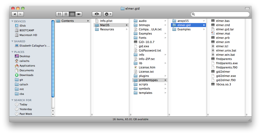
Here are steps I took to set up ElmerGUI. I'm running MacOS 10.6.8.

• Download ElmerGUI. Here's a guide to getting started with ElmerGUI.
  • Mac Looks sketchy, right? I swear it's ok.
  • Linux, or this, or this. (Can't vouch for these...)
  • Windows. (same story)
• Download GiD to create files for ElmerGUI.
• Set up GiD for Elmer export using Elmer templates for GiD. Download elmer.gid place it in GiD > Contents > MacOS > problemtypes.

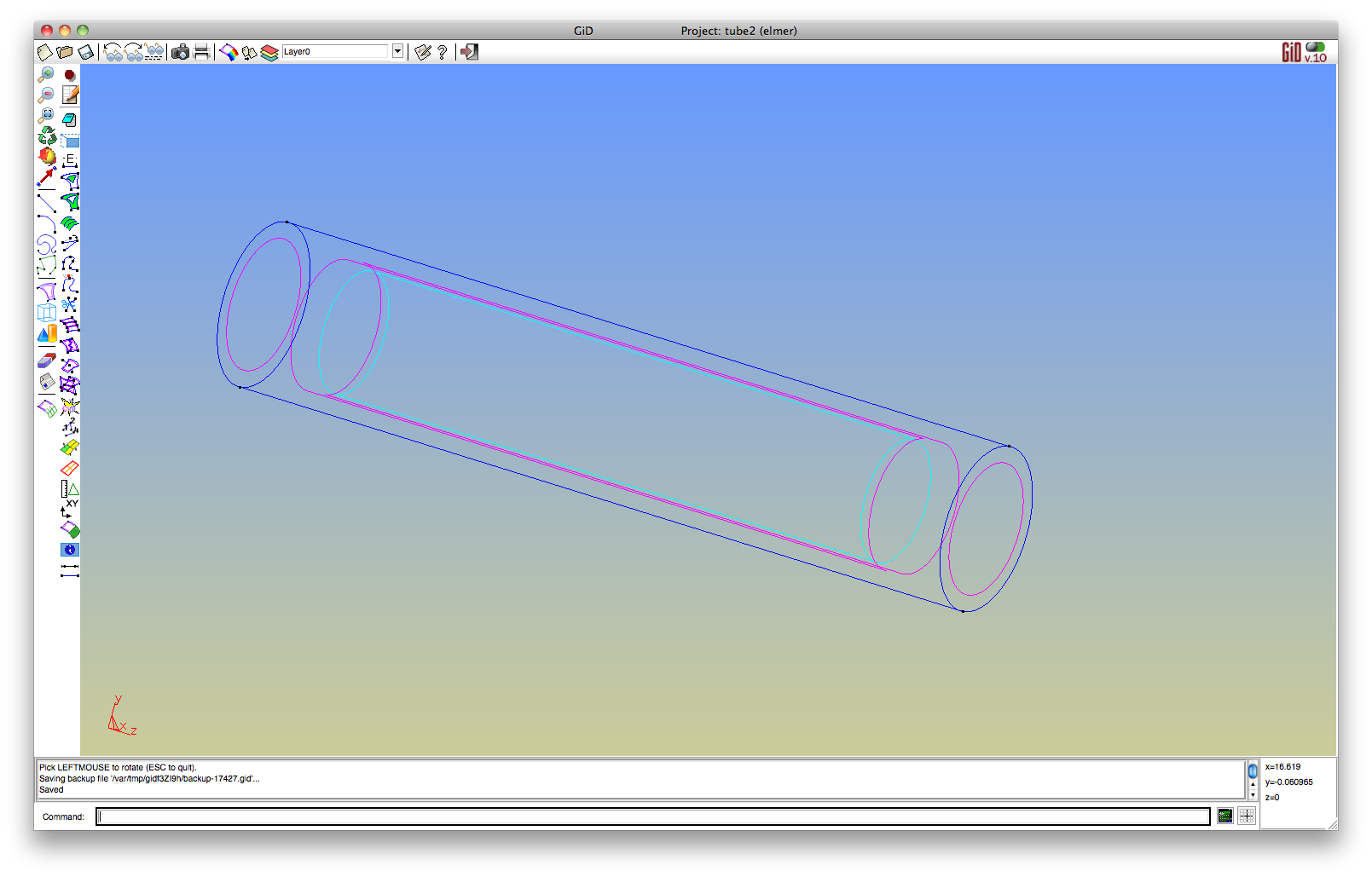
Get geometry into GiD. If possible, create it (by hand or with script) in GiD. There is import for meshes, IGES, 3dm, etc., but most meshes you meet on the street have all kinds of problems that GiD can't deal with.

Tell GiD about Elmer: Data > Problem type > elmer

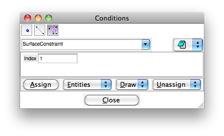
Now set up boundaries for conditions in Elmer: Data > Condition Because my boundaries are 2-d, I select the surface patch button. Click assign to select boundaries. Use as many indices as different boundary conditions that you want. In this case, I want two: a fixed surface and a free surface.

Similarly, assign bodies that will be associated with materials in elmer: Data > Materials > Assign > Volume If you're working in 2-d, this will be Surfaces.

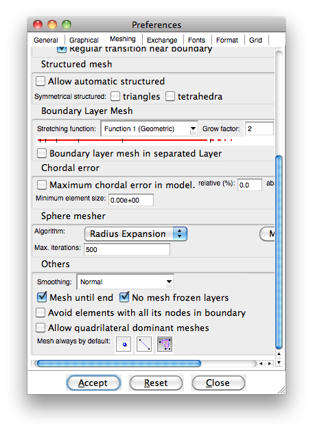
Now, very important: Utilities > Preferences > Meshing > Mesh always by default > Surfaces If you are working in 2-d, this will be lines. This is easy to forget, and if you do, GiD and elmer will silently fail to communicate.

Create the simulation mesh in GiD: Mesh > Generate Mesh The default element size should produce a reasonable but rough mesh. Experiement with finer meshes, but be aware that simulation times (particularly on volume meshes) can explode quickly.

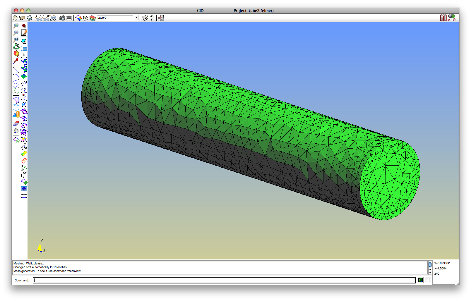
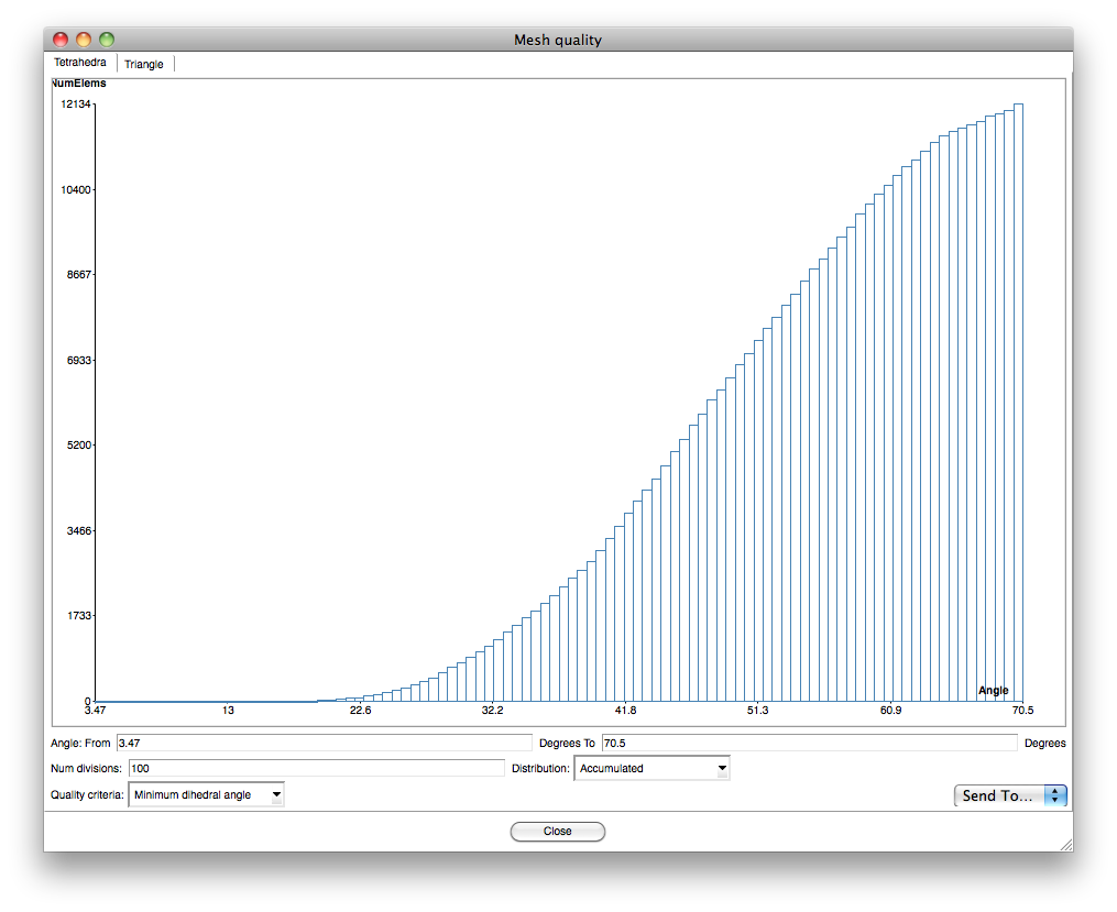
Notice its pretty isotropic, eh? How about that? You can measure that in Mesh > Mesh quality

The final step in GiD is to save the project, and run Calculate > Calculate. This will create the files for elmer to read.

To bring generated files into Elmer, under Configure in ElmerGUI, ensure the preferred generator is elmergrid (as opposed to nglib). Then click "Load Elmer mesh files" and select the .gid folder generated by GiD.

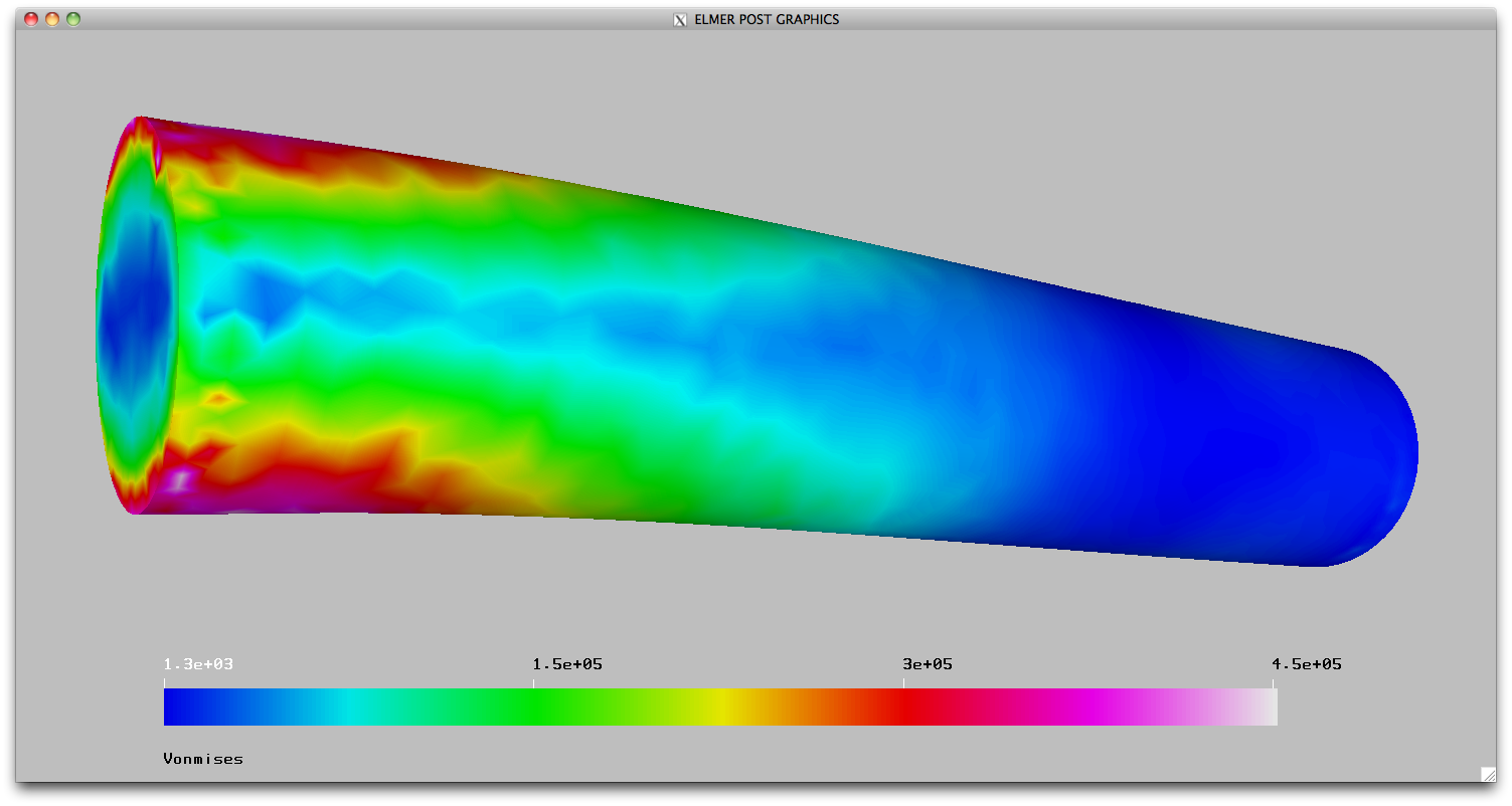
Now you need to assign model properties to the domain you created in GiD. You'll do this through the items in Model. Your problem will vary, but the top image on this page was produced with the following:

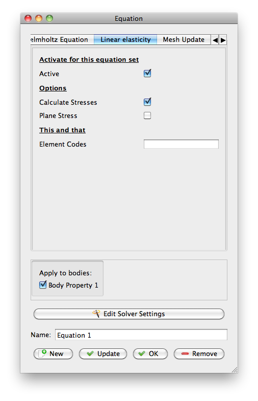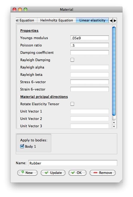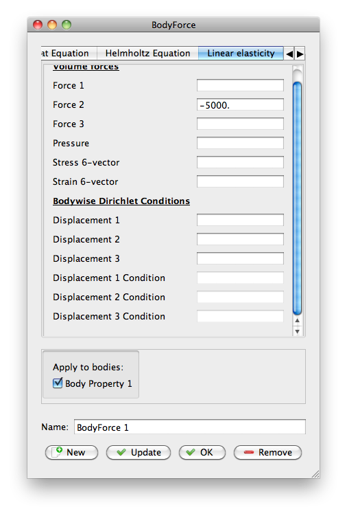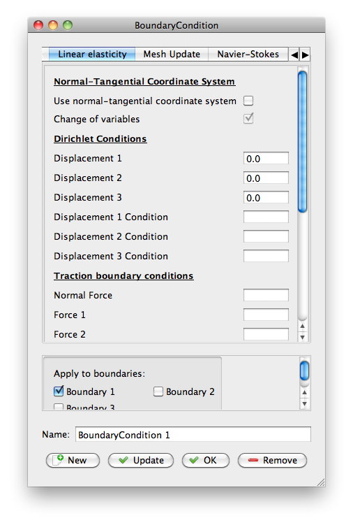Save the file, and Sif > Generate.

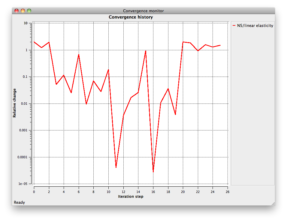
Now you're ready to run the sim: Run > Run solver You'll see a graph of convergence -- this can give you a clue if your sim is doing what you want.

You'll also see the solver log, which can be helpful to debug when your sim is not doing what you want.

 
: *** Elmer Solver: ALL DONE ***
SOLVER TOTAL TIME(CPU,REAL):       235.96      236.41
ELMER SOLVER FINISHED AT: 2012/11/29 15:28:47

To visualize the results of the sim, run the postprocessor, which contains lots of methods to show information over the domain.

• Solver log can hide behind convergence graph by default.
• After making changes in the GUI, you must always generate the SIF and save the project before re-running the solver with these changes (in this order!)
• To draw image in Elmer-Post, shifting nodes by Displacement, execute:

   
          math n0=nodes
          math nodes=n0+Displacement

Here's a sample SIF file. At this point, you should understand almost everything in it!

  Header
  CHECK KEYWORDS Warn
  Mesh DB "." "."
  Include Path ""
  Results Directory ""
End

Simulation
  Max Output Level = 4
  Coordinate System = Cartesian
  Coordinate Mapping(3) = 1 2 3
  Simulation Type = Steady state
  Steady State Max Iterations = 1
  Output Intervals = 1
  Timestepping Method = BDF
  BDF Order = 1
  Solver Input File = case.sif
  Post File = case.ep
End

Constants
  Gravity(4) = 0 -1 0 9.82
  Stefan Boltzmann = 5.67e-08
  Permittivity of Vacuum = 8.8542e-12
  Boltzmann Constant = 1.3807e-23
  Unit Charge = 1.60219
End

Body 1
  Target Bodies(1) = 1
  Name = Body Property 1
  Equation = 1
  Material = 1
  Body Force = 1
End

Solver 1
  Equation = Linear elasticity
  Procedure = "StressSolve" "StressSolver"
  Variable = -dofs 3 Displacement
  Exec Solver = Always
  Stabilize = True
  Bubbles = False
  Lumped Mass Matrix = False
  Optimize Bandwidth = True
  Steady State Convergence Tolerance = 1.0e-5
  Nonlinear System Convergence Tolerance = 1.0e-8
  Nonlinear System Max Iterations = 20
  Nonlinear System Newton After Iterations = 3
  Nonlinear System Newton After Tolerance = 1.0e-3
  Nonlinear System Relaxation Factor = 1
  Linear System Solver = Iterative
  Linear System Iterative Method = BiCGStab
  Linear System Max Iterations = 500
  Linear System Convergence Tolerance = 1.0e-8
  Linear System Preconditioning = ILU0
  Linear System ILUT Tolerance = 1.0e-3
  Linear System Abort Not Converged = False
  Linear System Residual Output = 1
  Linear System Precondition Recompute = 1
End

Equation 1
  Name = Equation 1
  Calculate Stresses = True
  Active Solvers(1) = 1
End

Material 1
  Name = Material 1
  Poisson ratio = .47
  Youngs modulus = 1.e7
End

Body Force 1
  Name = BodyForce 1
  Stress Bodyforce 2 = -5000.
End

Boundary Condition 1
  Target Boundaries(1) = 1
  Name = BoundaryCondition 1
  Displacement 3 = 0.0
  Displacement 2 = 0.0
  Displacement 1 = 0.0
End

Files:

• Mathematica Notebook with sim examples