My final project proposal this week is less of a project and more of a direction that I want to head toward. I'm not exactly sure what the implementation will look like (and even if I did, I think that would evolve a lot over the course of the next few months), so for this week I'm presenting some initial ideas and simulations of an concept I'd like to explore - amorphous computing.

Amorphous computing is a type of computational system comprised of many small, simple agents that can pass information to their immediate neighbors to produce global, emergent behavior. Some characteristics/necessities of amorphous systems include:

Local Interactions / Emergent behaviors - each agent in an amorphous network can only communicate with its nearby neighbors. The challenge of amorphous computing is to create meaningful emergent behavior from these local interactions.

Asynchronous - there is no global clock that syncs up the the agents in the amorphous network. This limits the assumptions you can make about the state of an agent at a given time

Global cooperation corrects errors in an individual - each agent in an amorphous system may have some error in its measurements, locomotion, or other functions. These errors should begin to vanish as you "zoom out" and observe the global behavior of the group. The presence of neighbors may also help an individual perform a task with lower error.

Self healing/error correcting/fault tolerance - Some agents in the amorphous system may fail completely and the system needs to be able to respond and adapt to these changes. The system should also be robust enough to work across various spatial topologies.

The thing that interests me the most about amorphous systems are their biological implications. Multicellular communication can be modeled as a type of amorphous system, so behaviors we observe in artificial amorphous networks may give us insights into naturally occurring phenomena. In fact, many tactics that computer scientists use to control amorphous systems are heavily inspired by biological processes: morphogen gradients, neighborhood query, local inhibition, local monitoring, agent differentiation, agent to agent contact (source).

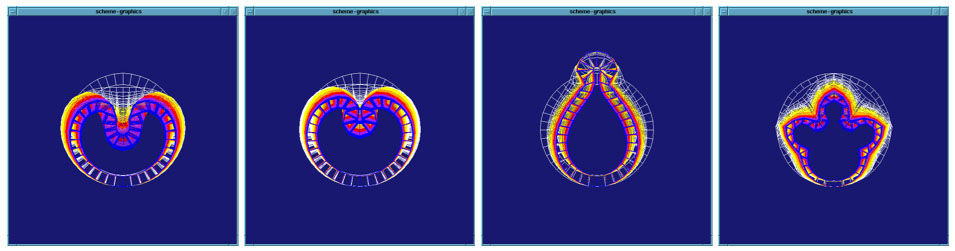
This paper by Radika Nagpal (with some figures from Odell, Oster, Alberch, and Burnside) demonstrates an amorphous mechanism for spatial cell arrangement and differentiation in the earliest stages of embryonic development, triggered by chemical gradients across a mass of cells (image below).

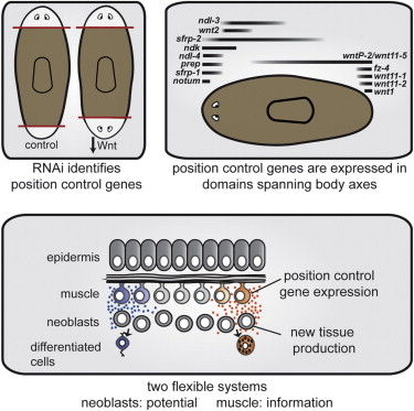
Planarians are small flatworms that have to ability to regenerate any part of their body. When a single planarian is cut in half, it may even regenerate into two separate planarians. This paper explain how gene expression varies across the planarian's body, forming a continuous gradient across the organism (image below). This gradient signals the regeneration of either a head or a tail (or some other part of the body), depending on how the animal is injured. Similarly, my first attempts at amorphous computing rely of the establishment and maintenance of a digital gradient across the system.

Some other interesting examples I've found include:

Bill Butera talks about the concept of a "Paintable Computer" in this thesis. He explains it best: "computation as a tangible, fluidly dispersible additive to ordinary objects. Want a surface to be smart? Add a layer of computing. Want it to be smarter? Add a second coat. Has the computing lost its luster? Get out the belt sander."

Kilobots are a very low cost (~$14 bucks per bot) platform for experimenting with swarm robotics. The bots can be programmed, charged, and activated in parallel, and they use a low cost IR technique for communication. This paper gives a nice introduction to the technology and ideas behind their design, more information (schematics, code, programming GUIs) can be found here.

The Simulation:

To start exploring this concept, I designed an amorphous simulation app in JavaScript. One of my goals for this class is to get more experience using JavaScript as a language for script-based, parametric CAD and modeling. I've done a lot of this type of thing with Processing, and have dabbled in a few other languages (Grasshopper/Python, OpenFrameworks, Objective C/iOS) to do 2D and 3D graphics, but I want to start using JavaScript so that my code can be easily accessed through the web. In my past life I was a content creator/developer at Instructables, and one thing I noticed there was that the act of downloading code and dependencies creates a huge (probably mostly mental) obstacle for people. If you want to engage your audience with a piece of code, you have to make it incredibly easy and accessible. I have come to the conclusion that JavaScript is the answer to this problem (for some things, there are obviously speed/memory limitations in the client side browser).

There are a few JavaScript libraries that make drawing in 2D and 3D on the canvas and exporting various file formats (svg, pdf, png, stl) much easier. Some that I've looked at include Paper.js, Easel.js, Raphael.js, Kinetic.js for 2D and Three.js/Three2STL.js for 3D. Though I'm pretty comfortable with JavaScript, I've mostly been working with more traditional UI elements (buttons, images, menus), so a lot this stuff is new for me. This week I'm using Raphael.js, but I'd like to explore the other libraries in future weeks (I picked Raphael for now because the API is relatively small and well documented). I'm also using JQuery for interactions with elements on the page and some helper functions, and JQueryUI for some custom UI elements (sliders, etc).

The app above demonstrates the perpetuation of a continuous line between end nodes, that does its best to maintain the shortest path between the nodes (measured by the number of agents in the path, not necessarily absolute distance). You can remove agents by clicking them, you can also click and drag the end nodes to move them - the simulation should correct for these changes. The rules for this app somewhat based off Robust Methods of Amorphous Self-Repair by Lauren Clement and Radhika Nagpal.

A few definitions from my code:

Agent - each circle in this simulation is an agent. Agents have a unique id number (created from a random number generator) and have the ability to communicate with their nearby neighbors. Agents store a few variables - state, hopCount, and successorId (defined below).

Nodes - Nodes are a special type of agent. Two nodes are included in the simulation, between which a line is drawn and maintained. They are called "node1" and "node2".

State - state is a boolean variable used to tell whether an agent is part of the line connecting the two end nodes. Agents with state = true are drawn in red.

HopCount - hop is a term from computer networking that refers to a node in a path that data is transmitted across. Each time a message is passed from agent to agent, a hop count incremented by one stored in the receiving agent. This sets us a gradient of hop count, radiating out from the origin of the message (hopCount = 0). You can see an agent's hop count by hovering over it.

SuccessorId - each agent stores the id number of its successor - the agent within communication range with the lowest hop number. This has the effect of saving a gradient across the system, where each agent is pointing in the steepest direction.

CommRad - commRad (communication radius) describes the maximum radius that messages from an agent can travel. The size of the commRad dictates how many neighbor agents a given agent can talk to. Dragging the "Communication Radius" slider shows an animation of what that asynchronous communication between agents might look like and gives you an idea of which neighbors are in range.

TransmissionNum - each message propagating across the system is attached to a transmission number. This ensures that hop counts from different transmissions do not get mixed and an agent can identify the more recent transmission.

Some assumptions/properties of my simulation:
- the time for a message to propagate through space is negligible compared to the time it takes for a message to pass from agent to agent. This may or may not make sense depending on the type of system you are modeling (for wireless communication between electronics, this makes sense). It would be interesting to see how this changes the establishment of a hop gradient across space.

- agent.state expires after a certain amount of time. This ensures that partial paths leftover by dead agents are removed in a timely manner. Maybe there's a more elegant way of achieving this effect, but it is a strategy I've seen in the literature.

-agents do not move. For the simplicity's sake (and to avoid crashing the browser) the position of the agents is static. There wasn't a great way for me to calculate the neighbor array in my simulation without doing a brute force check for the distance to every other agent in the system, so I didn't want to set my simulation up in a way where this would need to be recalculated continuously. In a real, physical amorphous system this wouldn't be an obstacle because the communication radius would take care of it for me. This is definitely a direction I'm interested in explore more.

-any outgoing messages must be sent to all neighbors. It is important to remember the physical constraints of the system I'm modeling; any messages that need to be sent to the successor will also be heard by the neighbors, so the neighbors must have a way to distinguish whether a message is for them. I did this by always including an id number in messages targeted towards a specific agent

Some things I've learned this week:

Sufficient communication radius - is it extremely important that agents are able to communicate across a radius large enough to reach at least 4 or 5 other agents. For sparse networks this becomes especially important. It was surprising to see how often my random spatial distribution of agents left some agents unreachable or created very awkward gradients around sparser regions. Communication radius also affects the rate that a message traverses space. This makes sense, but I hadn't considered the idea until I saw in in the simulation.

Conclusions:

I still have a few weeks before we get to the bulk of the electronics/networking section of the class, so I'm going to take this time to think about the specifics of how to physically implement some of these ideas. I'm hoping that the topics covered in this class and the "informal robotics" class I'm listening to this semester might help guide the direction of this project. I'd also like to expand on my simulation to quickly iterate on new ideas. Although my simulation is fairly simple at the moment, setting up a gradient in an amorphous system is the first step to performing other more complicated tasks, so it was useful to see how certain parameters affect gradient formation.