Week 4: 3D Printing and Scanning
This week, we were asked to design a 3D model and use the CBA machine shop's 3D printers to print these models. Additionally, we scanned an object of our choice using the Sense 3D scanner. I have some previous experience with geometric computing, so I decided to take a slightly different route in 3D modeling. I played around with the concept of 3d printed data and wearables that represent data, and ended up making a bracelet that represents the national anthem of Bangladesh (my country).
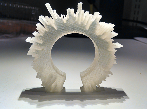
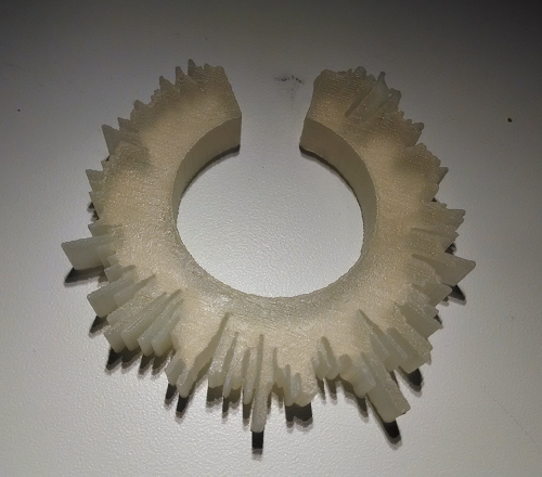
The end product, a national anthem bracelet:
Before diving into the details, here is a short version of what I did. I sang my national anthem into my microphone, took the waveform, plotted it, rasterized the plot, wrote some code to turn the raster into a 3D model that looks like a bracelet, and sent the 3D model off to the 3D printer in the machine shop.
How to Make a National Anthem Bracelet
Here's a hacker's way of 3d printing an anthem bracelet, using Mathematica as the math engine. The data preparation and 3D modeling took only two hours, but the method is more hacky than elegant.
Data Preparation
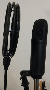
I recorded my voice using Audacity and an MXL-V63M condenser microphone in my home studio. A pop filter in front of the microphone prevents large pops ('p' and 't' sounds) and undesirable spikes in the waveform.
Then I imported the .wav file into Mathematica.
snd = Import["data/bangla.wav"]
Mathematica shows the waveform and spectrogram as the output.
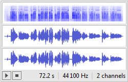
This a stereo (dual-channel) sound file, I had to take one channel's data and work with that.
mono = snd[[1, 1, 1]];
snd is a hierarchical data structure (called a nested list in Mathematica terms), the [[1,1,1]] part locates the data that we would like to work with.
A waveform is a list of amplitude values. I wanted to know how many such values were present in the waveform, so I could periodically filter out some data and work with a much smaller set of samples.
Length[mono]
returns the number of elements present in the list: 3184000. This is quite dense, so I decided to sample it by taking every 5000th value from the list.
mono = Table[mono[[i]], {i, 1, Length[mono], 5000}];
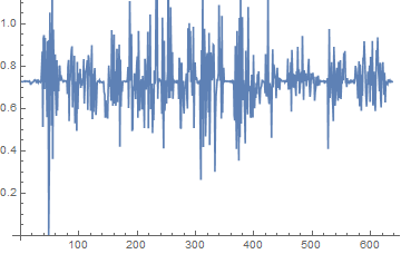
I subtracted the minimum value from all the samples values, so the waveform does not go below the origin (0, 0), and then plotted the waveform to examine it.
mono = mono - Min[mono];
ListPlot[mono, Joined -> True]
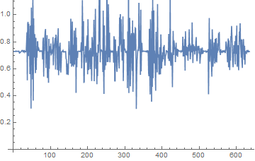
Even though I used the pop filter, there's an unwanted spike in the waveform. This could create a big partition in the actual bracelet, so I decided to run a cut-off filter -- removing values that are beyond a threshold amplitude value.
mono = Select[mono, # > 0.3 &];
ListPlot[mono, Joined -> True]
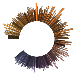
Rasterization
I decided to convert the waveform to a sector chart, and then rasterize the chart picture. For keeping things simple on the 3D modeling part, all values below the mean were reflected on the horizontal line that defines the mean. A sector chart is a circular chart, but I had to create an "opening" for the bracelet, so some 0 values were added at the end of the audio samples list.
mean = Mean[mono];
lst2d = Table[
   If[i <= Length[mono],
    {Abs[mono[[i]] - mean] + 0.05, mono[[i]]},
    {1, 0.0}],
   {i, 1, Length[mono] + 10}];

   md2d = SectorChart[lst2d, SectorOrigin -> {Automatic, 1},
  ColorFunction -> ColorData[39]]
Mathematica provides a function to convert any of its plots to a raster image.
rst = Rasterize[md2d, ImageSize -> 500]
With the rst variable holding the image of the plot, I ran some simple image processing commands. Binarize[] is a Mathematica function that takes an image and converts it to a binary image based on a threshold value. The default threshold value worked well for me, so I didn't play with the threshold anymore. Before running the thresholding filter, the raster image was blurred twice using the Blur[] filter, to get rid of sharp edges and threshold noise, and to make the structure look more organic.
bim = Binarize[Blur[Blur[rst]]]

Next, we copy the image data matrix to another variable.
bimd = ImageData[bim];
Generating the 3D Model
The 3D model generation is pretty straightforward. The following piece of code loops through all the pixels in the binary raster image, and creates a cuboid of fixed height if it finds a black pixel. The cuboids do not overlap since they have the same width and height (1 unit of length), so the polygon structure is tight and precise. Once we create a list of 3D primitives to be rendered, we can call the Graphics3D function in Mathematica that takes lists of 3D primitives and renders them.
gt = Table[If[bimd[[i, j]] == 0,
    {EdgeForm[Black], Black,
     Cuboid[{i, j, 0}, {i + 1, j + 1, 50}]}, {}], {i, 1,
    Length[bimd[[1]]]}, {j, 1, Length[bimd]}];


    gt = Select[gt, # != {} &];


    g3d = Graphics3D[gt];
The 3D model can now be exported to our desired format, .stl.
Export["g3d4.stl", g3d]
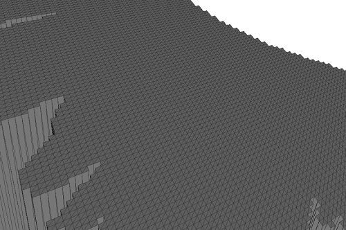
Using Meshlab, we can view the 3D model and its polygon structure.
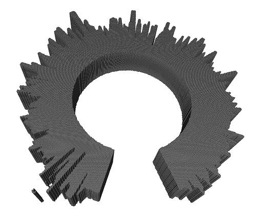
Note that there is an unwanted set of polygons that are detached from the bracelet structure. This is due to a small patch of black dot in the raster image that was generated during thresholding. I did not play around to get it correct, because after 3D printing we could always discard the extra part. The polygons do not overlap, and the mesh is nice and tight.
This is definitely not the best algorithm, as it produces a lot of unnecessary vertices and triangles. The STL file size was ~25 MB. I could write a better algorithm by combining connected components analysis and smooth meshing techniques, but for a two-hour long hacking session, this was good enough. The 3D printer does not care, as long as we don't feed it millions of vertices and triangles.
I sent the job to the Invision printer, and Tom Lutz helped me print it over the weekend. Since there were other people's jobs and time constraints, I had to agree to print a smaller version of the bracelet that would not fit my wrist. However, it would fit on a child's wrist, for now! I plan to re-print this to a scale that would suit my wrist, when everyone's done printing for this week.
There was some wax left after printing. I will need to use warm oil to clean this bracelet up.
Here's another view of the bracelet.
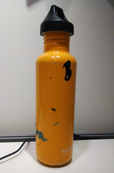
3D Scanning
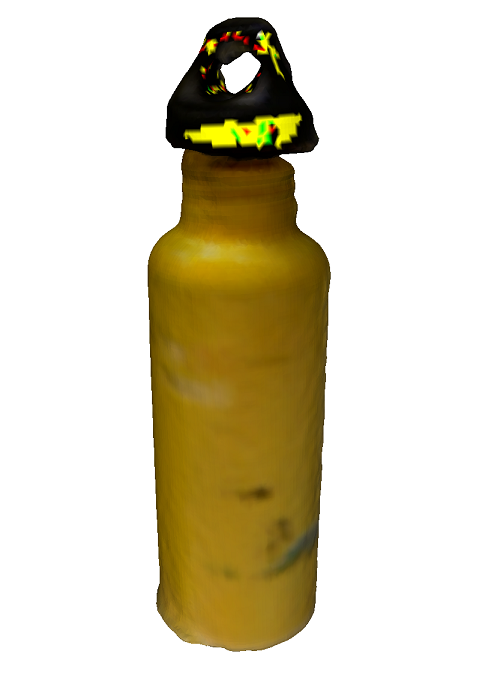
I tried several objects before I settled down to a solid water bottle for scanning. This was much easier to scan, as it does not have holes and openings.
After several tries, I could get most correspondences in the scanned images to match up using the Sense software. The model was exported to .obj format to preserve the color information. Using Meshlab, I cleaned up some noises and unwanted surfaces present in the 3D model.
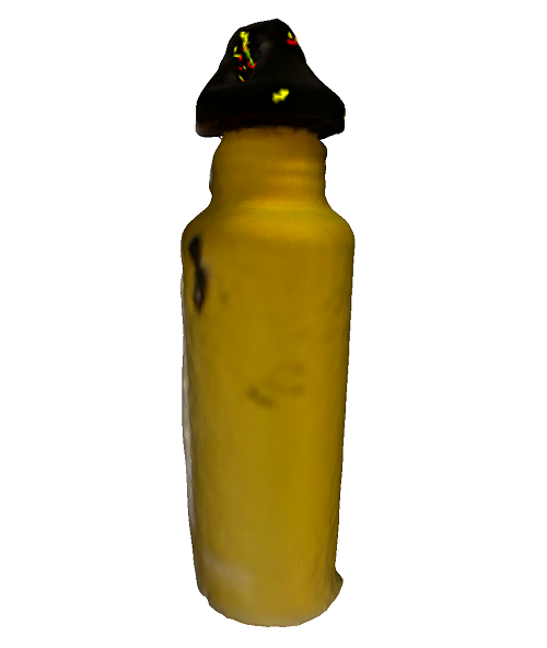
I was able to capture the cap precisely, but the software could not reconstruct the colors properly. This must be due to lack of feature correspondence data, which means I simply had to take more sample frames.