Week 3: 3D scanning and printing

This week the two assignments were to 3D scan an object of our choice using the Artec 3D scanner and characterize, model and print a form of our choice that couldn't be done by CNC milling a subststrate.

3D Scanning

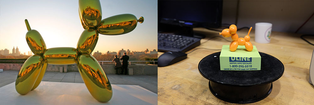
For the 3D scanner I choose to scan a miniature toy I have that is based on Jeff Koons sculpture. The reason for the choice was based on the fact that the physical object has a very plastic, 3D light aesthetic. I thought it could be interesting to use it. I used the Artec Scanner and before I could get better scans I had some failed attempts. Mainly for positioning the scanner too close to the subject. I found that a distance of 1 meter away is ideal. I placed the toy on the rotating plate and used a green stack of post it notes to give a floor to my scan.

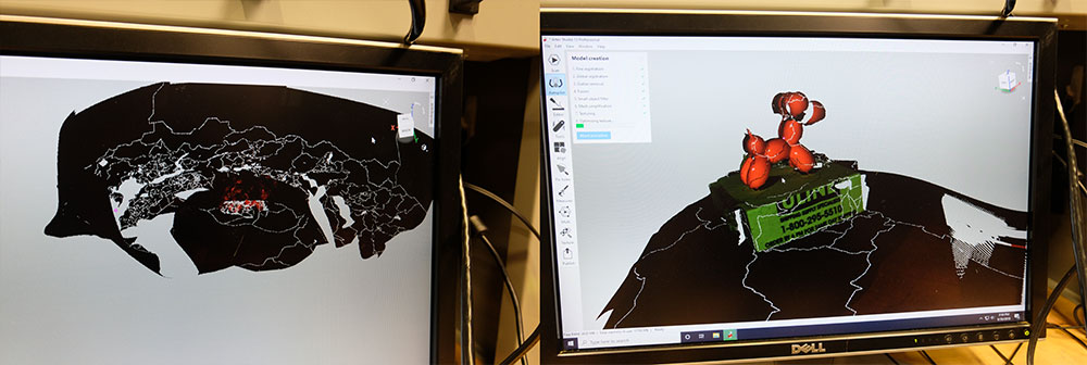
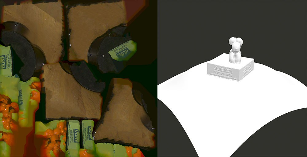
The image above shows my initial failed attempts to scan using the Artec and positioning the scanner too close to the subject. After a few attempts I started getting better images. I also tried by scanning over 800 frames (letting the object spin for a long time), the issue I encountered was the software crashing. Following Tom's recommendation I found that 1m distance of the subject, steady hand and let the object spin once was the ideal to get good scans.

To export it from the ArtecStudio software I used the OBJ format as I wanted to have the mesh and the texture map for my model. Below you see a video of me moving the OBJ around on OSX. Note that the 3D scan includes the stack of post it notes and a mesh for the table.

I then imported the OBJ file into Rhino and used the Lasso tool to remove unwanted parts of the background and rendered the images below. I noticed that the scanner is very accurate in representing the volumes and mapping them to textures, but I could see quite a lot of noise in planar surfaces (such as the green post it notes below the toy. I was also impressed on how accurately the texture is mapped on the 3D geometry wrapping it in the correct colors and textures.

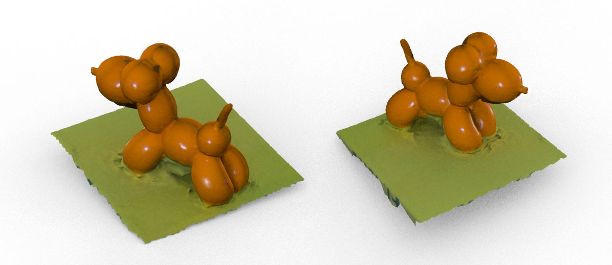
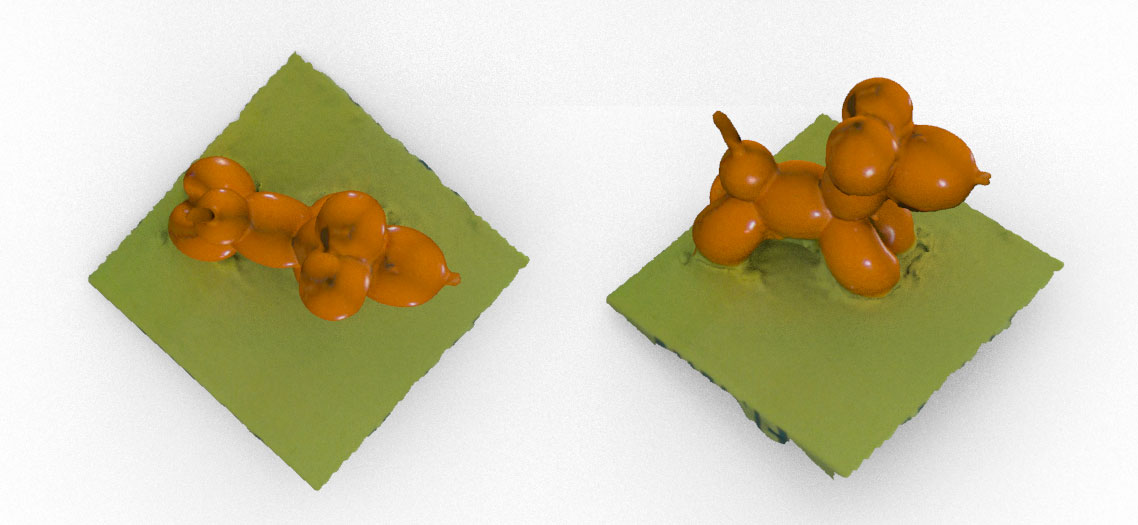
Here is a side by side image of the mesh and the texture that is mapped on to it. This image shows the geometry and texture prior to importing the file into Rhino and using the Lasso tool to remove the background and rotating base.

3D Printing

Characterizing Conductive Inks

For the 3D printing assignment I decided to make it in two parts. I have always been interested to characterize the conductive filament on a 3D printer. So in partnership with Alfredo, we both designed a series of geometries to be printed using 2 distinct conductive filaments in the Prusa printer. Instead of characterizing the printer we did on the material.

The idea behind this was to explore what are the best ways to 3D print conductive filament. The first filament tested was the Protopasta Conductive PLA and we then tested Electrifi Conductive Filament recommended by Juliana Cherston as one of the best ones out in the market.

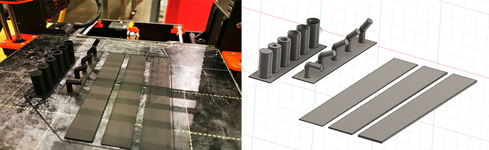
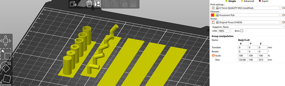
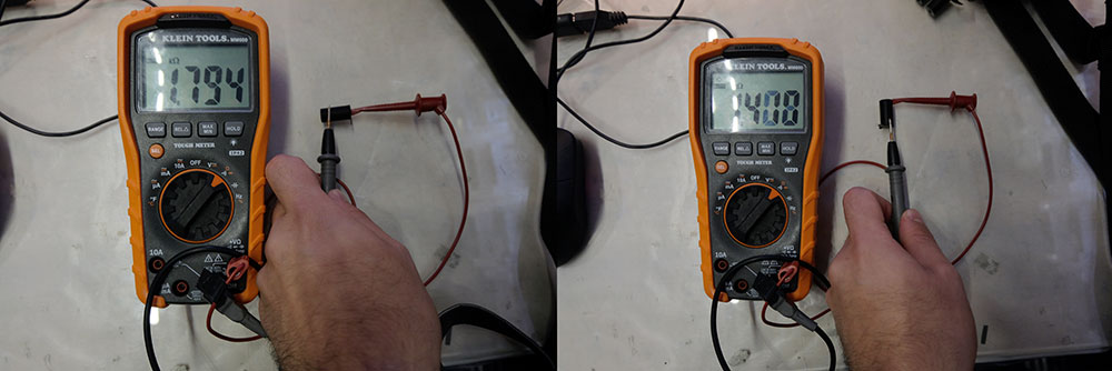
We 3D printed the structures using the Prusa Silcer with the settings below. Altough the prints chame out as expected, we tested the conductivity with the oscilloscope and the result was really poor. On the solid pipe we could see around 40KOhm resistance when measuring the pipes with a multimeter.

We then moved on to experiment the Electrifi filament. We followed the recommended specifications of printing with a 0.8 nozzle size (we switched the nozzle of the Prusa) and 160 degrees nozzle temperature. We had a series of issues where the Prusa just wouldn't print (we could see that it wasn't pulling the filament). After a number of attemps we found that if we set the temperature to 200C on the GCode file we then could print successifully.

Despite the manufacturer statment about the conductivity we found the filament to be very unreliable, the resistance wouldn't be constant. At this stage I decided then to move on to another idea using normal filament. I still plan to get back to experiment with conductive filament, but for now I focused on doing something I could achieve by next class.

3D Printing Real Time Data

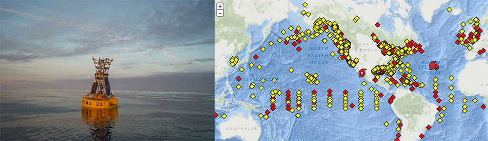
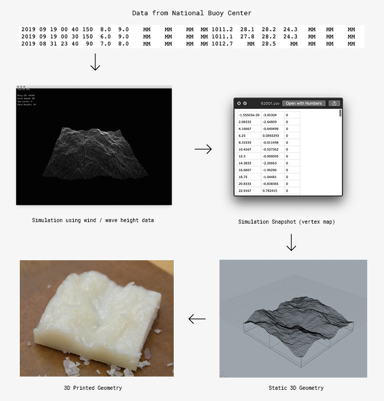
A few months ago I wrote a simple program to capture real time (ish) data from ocean weather buoys. This data can be found in the NDBC NOAA website in the form of text based lists that you can access from buoys around the world. This is an example of a data feed.

I was curious to create a simple simulation that could emulate a section of the sea in any part of the world by simply reading real time data about the wind speed and wave height from this feeds and mapping that into a simulation.

For my assignment I decided to revive my code for this idea and take a snapshot in time of multiple buoys and turn that dataset into a physical artifact.

For this experiment I connected my application to the feed of 3 buoys:

Station 62001 - Gascogne Buoy 45°13'48" N 5°0'0" W
Station 44139 - Banqureau Banks 44°14'24" N 57°6'0" W
Station 64046 - K7 Buoy 60°29'0" N 4°10'0" W

I used Python to write a webservice to grab the text file from the NOAA service and parse it into an object. I then used OpenFrameworks with the ofxOcean addon. On the video below I switch between three buoys (note the id changing) and you can see the different portions of the sea at that given time.

I then exported the vertices of my simulation to a CSV file and with the help from Jake (that wrote an Grasshoper script to turn my vertices into a clean mesh) we created a little block that represents the ocean at that given point in space and time.

Prior to using Grasshoper I attempted exporting the mesh directly from openFrameworks and cutting it with Fusion360. The issue was that the exported file contained a series of overlapping vertices which made it hard to render the shape.

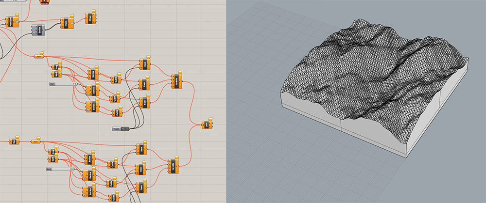
Jake's Grasshoper script read in the CSV exported in openFrameworks and iterated over the ordered list of vertices by drawing triangles on both directions, by doing that we created a mesh that is the surface of the vertices. We then extruded that as a solid block and gave it some height.

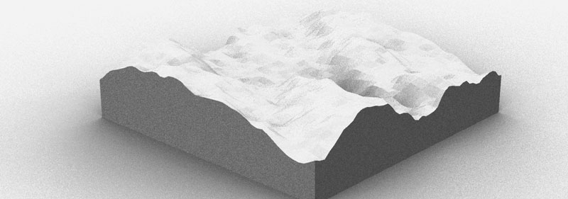
Below is an image of the pipeline I developed to produce the 3D printed object. I used data from the National Buoy Data Center to drive a fluid simulation based on wind speed, wave height and ocean height parameters. I then took a snapshot of the simulation at a given point in time. I exported the snapshot as a CSV with vertices. Using Rhino/Grasshoper (thanks to Jake) the CSV data is rendered as a mesh that I then exported as STL and 3D printed.

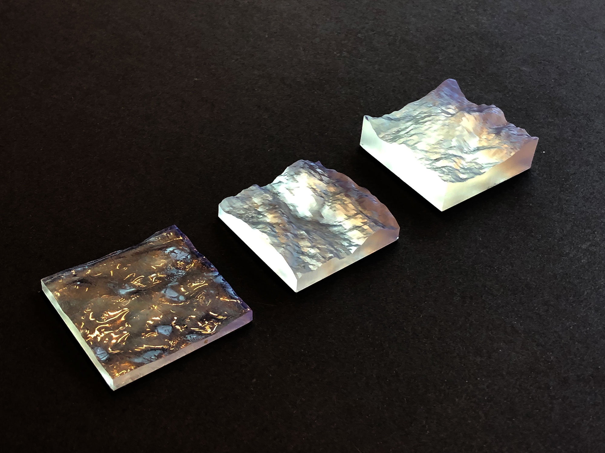
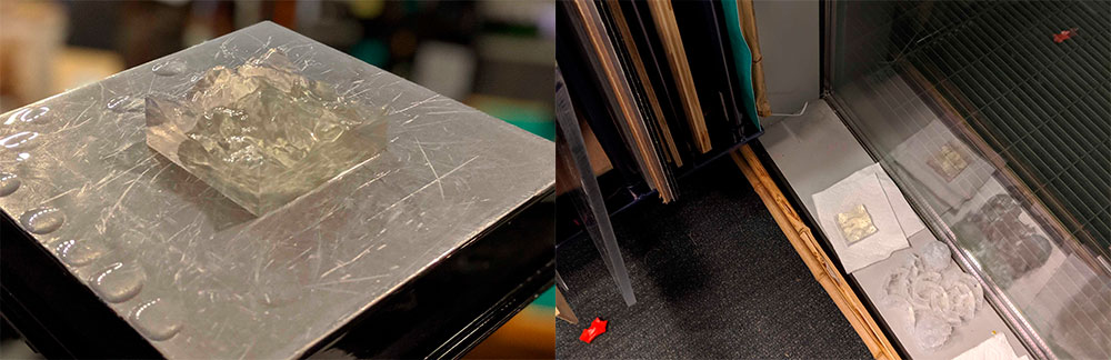
Here is the final result of the parts printed using Formlabs and Clear resin. Here is the Formlabs result being taken out of the printer.

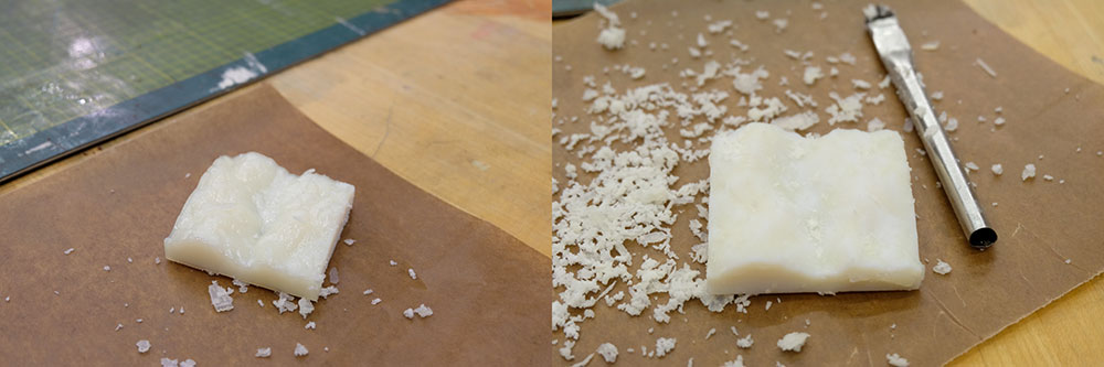
Here is the 3D printed bit of ocean.