Intelligent Audio Segmentation and Quantization using Dynamic Programming
This document explains Jeff Lieberman's final term project for
the class 'The Nature of Mathematical Modeling,'
taught by Neil Gershenfeld at
the MIT Media Lab in the Spring of 2oo5.
Abstract:
Typically, attempts to work with rhythmically precise audio patterns involve the use of either MIDI
[musical instrument digital interface], and therefore MIDI quantization, or the use of a live 'click track'
by which the live performer can gauge their performance in real-time. Herein is described a method,
designed to work in real-time, to record a live audio performance, without the need for an external
click-track; the method fixes audio data by first segmenting it into constituent parts, and then aligning
these parts to a 'goal tempo', with the option of using a style template to help align a performance
to a specific genre of music. This method of intelligent quantization allows a wider variety of
musical environments to be captured and aligned for use in recordings: specifically, this allows the
use of captured data from live performances or in studio situations, to be tranformed into manageable
and useful entities for production quality audio.
- Problem/Scope and Approach:
There are many situations where capturing the audio of a live performer/performance would be
useful; either for future studio work, or in fact for the live performance itself. However, in most of these
situations, performers will make mistakes. The most typical mistakes happen when the performer has a
false start, or when the performer gets ahead or behind the beat. This occurs even when in studio
situations, when the performer often wears their own pair of headphones which provide a 'click track'-
a marked tempo metering. Often valuable studio time is spent/wasted when a performer plays something
of difficulty, as they need to repeat it over until getting it just right.
When a performer uses MIDI [the musical instrument digital interface], their notes are captured as a
series of 'note on' times, with velocity values. The computer synthesizes the notes in real-time regardless
of when they were originally played. Therefore, quantization is intrinsically easily accessed tool. However, two
problems exist with live audio: First, the audio does not exist in a simple segmented form with which to
quantize, and secondly, quantization of audio or midi is typically done by finding the nearest neighbor in
whatever subdivision the user chooses. This simple algorithm is useful, but not ideal, for it cannot fix the
most common mistake in audio performance - subtle shifts in tempo over time, which cause the audio to
fall in front of or behind the actual beat. An example is shown:
As is easy to see from this example, typical audio quantization produces a massive shift in perceived sound:
what was once a perfectly regular beat, albeit played too slowly, has become a massively irregular pattern.
Thus, we search for a way to input audio from a performance, first segment it into parts, and then align
these parts that in some way preserves the 'spirit' of the performance as best as possible.
- Audio Segmentation:
The first task we must perform is to take an input audio track, and split it into parts where rhythmic
events occur. At first glance this problem appears in some ways trivial, and in some ways intractable. First,
in many rhythmic samples, complete silence proceeds a rhythmic event. But often, one event has not finished
when the next event occurs. Therefore we require slightly more sophistication then merely searching for
zeros in segmenting the audio track into parts. Most of this analysis was first performed by Tristan Jehan
(see Event-Synchronous Music Analysis/Synthesis, Proceedings of the 7th International Conference on Digital Audio Effects [DAFx'04]. Naples, Italy, October 2004), although slight modifications have been made for robustness
and higher frequency rhythmic content.
Below is a picture of the segmentation process [click for larger view].
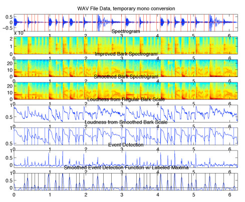
There are four stages in segmentation.
- Time/Frequency Analysis: First, a STFT (short time fourier transform), also known as a
spectogram, is made of the audio signal, at roughly 3ms windows [while padding the windows to allow
for wider frequency spectrum content]. This allows us to analyze the audio in both the time and frequency
at the same time. However, the even breaking of frequencies in the audible range does not correspond
with human perception; humans possess critical bands of frequency perception that stretch wider with
rising frequency. Thus, we convert the equidistant audio spectrogram into one by a human scale. This is known
as the Bark Scale.
- Temporal Masking: Humans cannot perceive a loud then soft sound in the same frequency when the time
between them is too small, roughly 150ms. Thus, we convolve half of a hamming window [ie. raised cosine window]
with the Bark scale spectrogram, in order to give us a more 'human perception' measure of sound attacks. This
also helps reduce noise in the signal, to lower the risk of false positives.
- Energy Content/Loudness analysis: We then sum the energy in each frequency band to get a measure of
human perceived energy over time. This is our loudness spectrum for the track. Sudden rises in this spectrum
are our attacks in the audio sample. By taking the discrete derivative of this, we find that peaks associate with
these sudden maxima.
- Trackback: We use these cues of attacks as starting points to look for exact attacks in the audio sample,
and we make sure to find the exact frame at which the attack range leaves zero, to thus remove any clipping.
- Audio Quantization:
Typical audio quantization is usually very effective, when the performer plays close enough to the original
tempo that they are never more than half of the grain size mistaken in their playing [i.e. if quantizing to an eighth
note, they must never err more than a 1/16th note]. However, if given a sample of someone playing in an unknown
tempo, aligning it well enough to a click track for quantization to work properly becomes a very difficult task. We apply here a more rigorous method to aligning tracks that frequently possess these problems.
The approach that we employ here is to set up a set of cost functions that we consider good gauges of musical alignment in a sample. Given a set of attack original times {t} and associated weights of their attack {w} (measured as the maximum total energy in that sample), and a set of possible template times {templateTimes} with their associated weights {templateWeights}, the first of these is the completely typical quantization scheme: an attack would like to move as little as possible to be in the correct place. This is represented by our first cost function,

Note here that i represents our current point.
The second cost involves these template weights. An optional input is a template weight set, which indicates the
probability of notes hitting at certain times in certain genres of music. This allows a user to weight a certain template scheme, to enforce a style even if the player was far from matching that typical style. This cost is measured simply as:

The final cost is the main addition that allows us to fix massively imperfect recordings, and bring them to perfectly stylized and rhythmic form [at any tempo]. The observation is that, in general, the performer will overall be trying to play at some distinct tempo, and may fall behind or ahead of the beat, but in general will do so over medium distances in time, not instantaneously. Said another way, their mistakes will mostly be subtle with respect to timing, not jerky and obvious. How do we measure this? One way is to measure the local accelerations at every possible point, where here we refer to accelerations as the way that we have altered the original times to bring them to quantized times. For example, if a performer played two notes quickly in succession, and then one after a break, if we quantize these to all be equidistant on the time axis, we will have decelerated time for the first pairing, and accelerated it for the second. By choosing a cost function to minimize only the changes in these accelerations, we allow for performances to slowly completely lose track of the beat, as long as they are somewhat consistent with themselves. This cost is represented formally in the following:

Finally, we sum all of these costs using weighting parameters to determine how important each cost is. These are variable in real time use, so can be tuned for separate examples if the user knows the sort of audio they are dealing with. The final cost for a mapping selection is the sum of individual point costs, represented as

- Approach using Dynamic Programming:
In a small set of possible rhythmic points and possible template matches, the ideal solution to this problem would be a simple iteration of all possibilities and their costs, as it is trivial to compute and takes no thought/effort. However, a simple audio sample of 4 measures [16 beats] has 64 possible template points, and roughly 20-40 attacks [let's assume 30]. This possesses roughly 1.6e18 possible combinations. Using a gigahertz computer, and not accounting even for the costs involved in calculating the cost function, this will still already be an intractable problem, taking over 50 years to compute. However, we want this to function in real-time! This is where dynamic programming saves the day.
The event placement routine of which we are trying to minimize the cost is a perfect routine to exploit dynamic programming. We can represent the choice of any step recursively based only on previous choices [in our case, we only need to keep two levels of history given our cost functions; the current step location is notated as i, with the previous step j and the step before that k]. All future decisions are made independent of the path by which they arrived, as long as they arrived at location i. If we can minimize the cost of any step, based solely on placements of previous steps, we are ripe for dynamic programming. This is known as the principle of optimality, and we will exploit this below.
Let, as mentioned above, our current step (i) assumption be that it lays at template time templateTime(i). Previous steps j and k are allowed to rest at earlier template times. For every step we make the following iteration:
- For step = 1:totalSteps,
- For i = step:totalTemplateTimes,
- For j = step-1:i-1,
- For k = step-2:j-1,
- Generate the cost function of these possible choices, and add it to any previous minimal cost to
arrive at this location.
- Find the minimal choice (with respect to k) to bring us to this path of j and i.
- Save this local cost.
- Over all choices of k, find the total cost so far for the pair (i,j) for this step.
- Set the previous best choice given (i,j) to be k, for tracking backwards.
- Trackback:
- Start at the last point, and find total minimum cost.
- For each previous point, find the minimal cost that will let us arrive at the next point, and choose this
value.
In this way, we are able to step through forward and then backward, and by only judging local costs, find the minimal global cost minimization scheme. Not only that, but this can happen faster than the sample is played, ie. can be utilized in real-time analysis.
[Note: there are special cases for step == 1 or 2, since there is no valid way to step backwards with both j and k].
- Combination / Results:
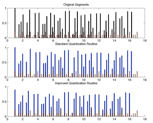
Below shows two examples of this intelligent quantization scheme, on two sets of data. The second and more complex example shows a situation where the beat was mostly consistent, however it was performed slightly slower overall than the tempo. Therefore typical quantization schemes fail miserably at this; in this case the regular quantization scheme produces the incorrect solution for over half of the sample. This example is shown in audio clips below.
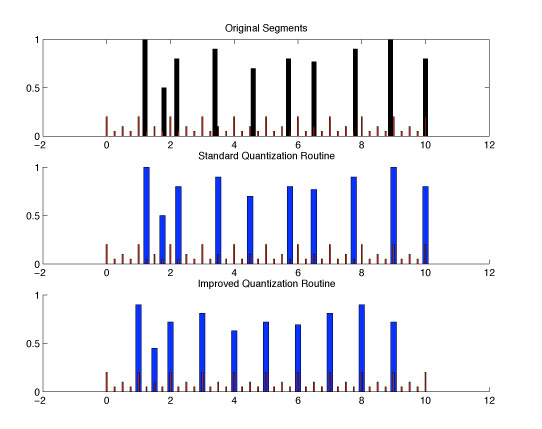
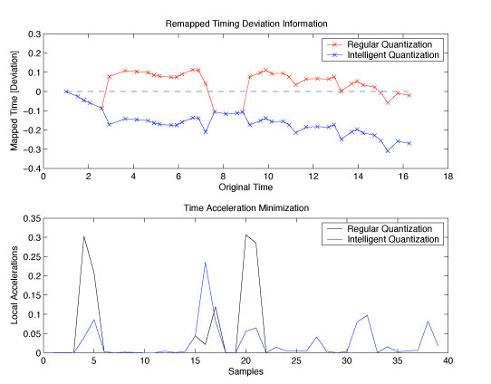
The graph below shows specifically the results of this new acceleration minimization cost. The top subplot shows deviation from the original times of each sample, where the blue shows the improved version. Note that since the sample needed to be slightly sped up, the blue track slowly deviates from the norm, whereas the normal quantization scheme, by definition can never leave that region. The improved scheme captures what is obvious to any listener of the original sample, as to the goal of the performer. The second subplot shows the time accelerations for each scheme; as can be seen, indeed, this new scheme lowers the overall amount of local accelerations.
- Audio Samples:
What would this research be without audio samples to show its ability. Below is a sample track of Eric Gunther beatboxing one loop, however, slightly behind the beat [which I've added as a click track in the two processed versions]. The
Here are the matlab routines that run this code:
All material copyright 2oo5 Jeff Lieberman.
|
