Finite Differences: Ordinary Differential Equations
The majority of my time this week was spent going through numerical analysis reference materials before directly
tackling any of the problems. My major goal this week was to gain an intuitive understanding of Runge-Kutta methods
and why it is even better than Euler's approach.
(1) What is the second-order approximation error
of the Heun method, which averages the slope at the beginning
and the end of the interval?
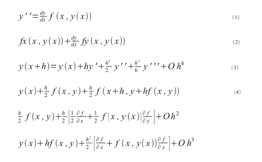
Thought process: I start out with equation (1) where points (x, y) are approximate solutions to the
differential equation. Then apply the chain rule for equation (2) to express Taylor's formula to obtain a useful
estimate on the error term (3). The Huen method (4) expands and generates into an iterative scheme that first
predicts and then corrects for y(x). Expanding the last solution is similar to equation (2), there are no errors here.
(2) For a simple harmonic oscillator y:+ y = 0, with initial conditions y(0) 1, y:(0)=0, find y(t) from t = 0
to 100 * Pi. Use an Euler method a fixed-stepped fourth-order Runge-Kutta method.
After trying out the Runge-Kutta method by hand, I moved onto translating the method in Python and Java
The thought process is outlined in the following code: rungekutta.java
with these results:
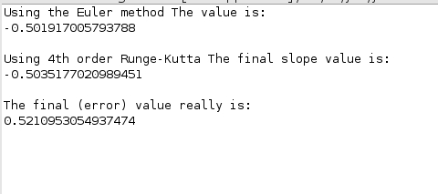
The results strayed from what I had predicted. My goal was to obtain an intuitive development for the derivation
of the fourth-order Runge-Kutta method. That is, the first estimate of y comes from Euler's method. The factor of 1/2
comes from a step size from x0 to the midpoint - to correct the estimate of y at the midpoint, we calculate again.
To predict y1, we use Euler's method. The Runge-Kutta scheme is obtained by substituting the estimates into
y1, giving us 4 points along the curve. This technique gives very accurate results without the need to take small steps,
or values of h. Euler's method on the other hand, is obtained from approximating the integral where y1 = y0 + hf(x0,y0).
Continuing in this fashion are points of the approximate solution, where the aggregate error is bounded by the step size (h)
and some constant.