Transforms: Wavelets, PCA, ICA
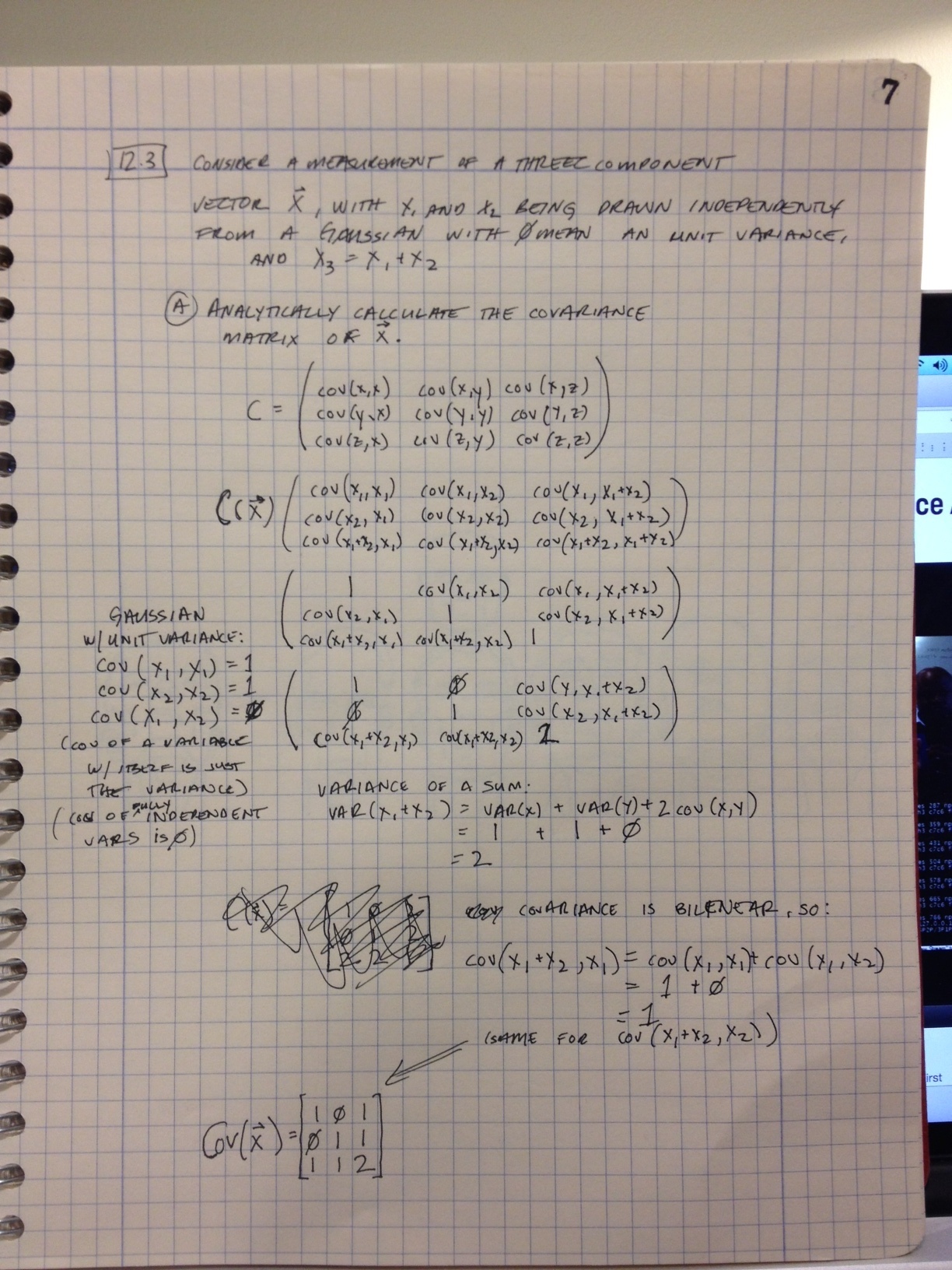
12.3) Consider a measurement of a three-component vector x, with x1 and x2 being drawn independently from a Gaussian distribution with 0 mean and unit variance, and x3 = x1 + x2.
a) Analytically calculate the covariance matrix of x
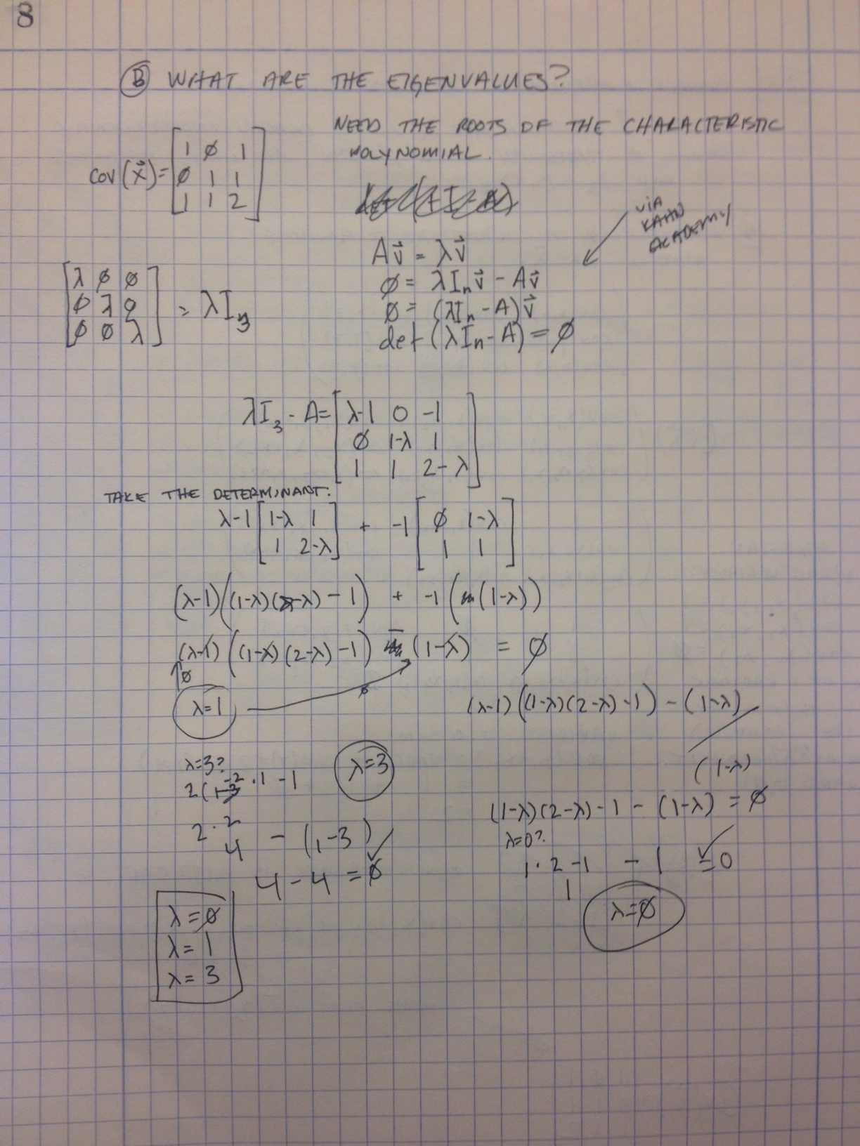
b) What are the eigenvalues?
C) Numerically verify these results by drawing a data set from the distribution and computing the covariance matrix and eigenvalues.
Code here: pca.py
import numpy as np

n = 100000

x1 = np.random.normal(0,1,n)
x2 = np.random.normal(0,1,n)
x3 = x1+x2

X = [x1,x2,x3]

c = np.cov(X)

print(c)
# Covariance matrix:
# [[ 1.00552305 -0.00540942  1.00011363]
#  [-0.00540942  1.00327819  0.99786877]
#  [ 1.00011363  0.99786877  1.9979824 ]]


e = np.linalg.eig(c)
print(e[0])
# Eigenvalues:
# [  2.99277382e+00   1.00136031e+00   1.76529821e-15]
D) Numerically find the eigenvectors of the covariance matrix, and use them to construct a transformation to a new set of variables y that have a diagonal covariance matrix with no zero eigenvalues. Verify this on the data set.
Continuing the excerpt of pca.py above:
  print(e[1])
  # Eigenvectors (col major):
  # [[-0.40445603  0.70928273  0.57735027]
  #  [-0.41202885 -0.70491056  0.57735027]
  #  [-0.81648487  0.00437217 -0.57735027]]

  # Cov(y) = M * Cov(x) * M^T
  cy = np.dot(np.dot(e[1].T,c), e[1].T)
  print(cy)
  #
  # [[ 2.61908171  0.80509741 -0.50471862]
  #  [ 0.80509741  0.98241759  0.30643185]
  #  [-0.50471862  0.30643185  0.38716296]]
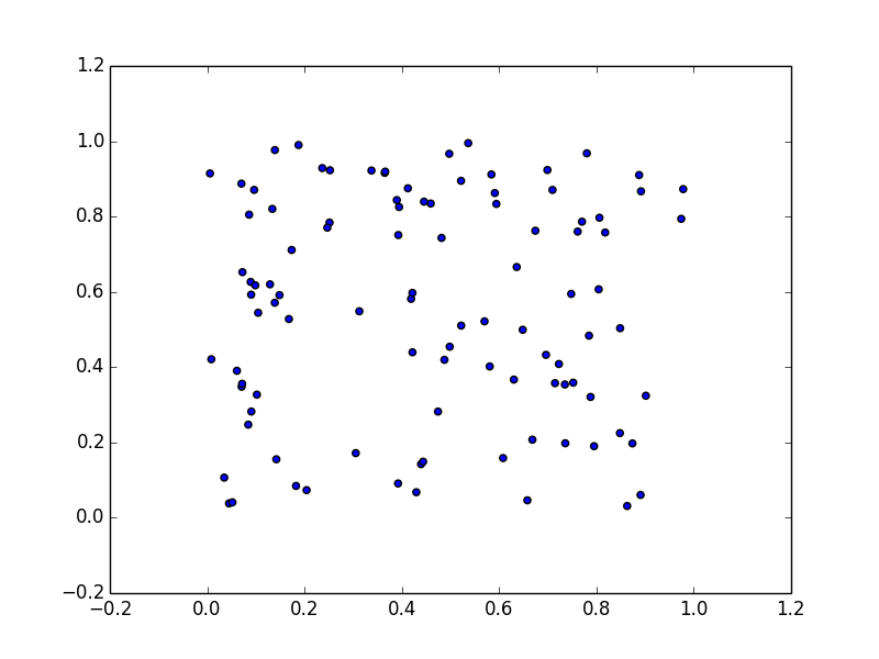
12.4) Generate pairs of uniform random variables {s1,s2} with each component contained in [0,1].
a) Plot these data.
Code here: ica.py.
import numpy as np
import matplotlib.pyplot as plt

n = 100

s1 = np.random.uniform(0,1,n)
s2 = np.random.uniform(0,1,n)

plt.scatter(s1,s2)
plt.show()
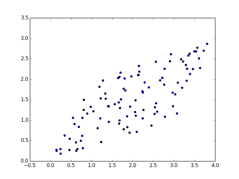
b) Mix them (x = A*s) with a square matrix A = [[1 2] [3 1]] and plot.
Continuing from ica.py...
S = np.column_stack([s1, s2])
A = [[1,2],[3,1]]

mix = np.dot(S,A)
plt.scatter(mix[:,0], mix[:,1])
plt.show()
c) Make x zero mean, diagonalize with unit variance, and plot