Final Project: Molecular Simulations of Lipid Membranes
James Pelletier
MAS.864 Nature of Mathematical Modeling
Question: How to insert big molecules into biological cells?
This figure shows an image from my research project - these are bacteria about 1 micron in diameter. The fluorescence signal shows whole chromosomes, initially outside the cells. Our goal is to push the chromosomes into the bacteria. At the start, the chromosomes appear like rings because they coat the surfaces of the spherical cells, and through the microscope we view a projection of the system.
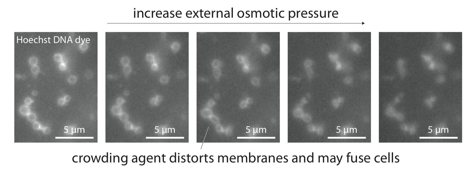
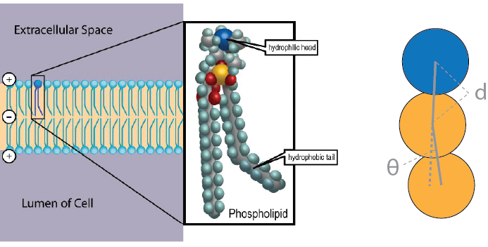
I have several interests in lipid membranes, the dynamic structures that contain and subdivide biological cells. Lipid membranes are semipermeable: many small molecules can diffuse through membranes; however, highly charged molecules such as DNA cannot pass through the hydrophobic barriers. In order to install DNA in cells, we must transiently open holes in the membranes. Transient electric fields and osmotic shock can permeabilize cells. Chemical treatment with divalent ions followed by osmotic shock can even push enormous pieces of DNA (megabases) into bacteria (about 1 micron in diameter), or fuse bacteria together. I would like to gain some intuition for the mechanisms that govern hole opening/closing in membranes and transport of materials through the holes.
In particular, how do osmotic pressures rupture membranes? How large are the holes? For how long do the holes live?
Prior art
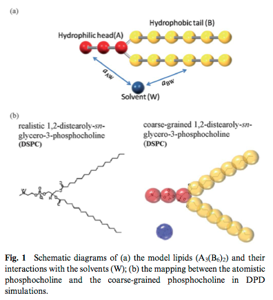
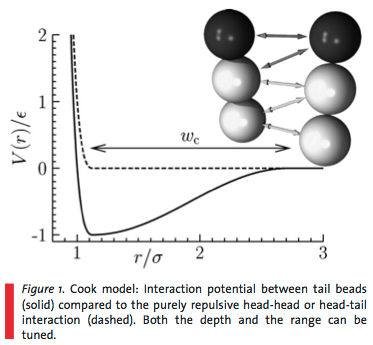
Due to the molecular complexity of the biomolecules, atomistic simulations are limited to 10s of nanometers and a few nanoseconds integration time. Furthermore, membrane structure is a function of solvent quality - and explicit inclusion of all the solvent molecules costs a lot of computational effort. Therefore, I have been reading about coarse-grained, solvent-free molecular dynamics simulations. "Coarse-grained" means we simulate minimalist molecular models to reduce the number of degrees of freedom and focus in on the core physical phenomena (Figure 1).
"Solvent-free" means we do not explicitly include the solvent molecules; rather, we implicitly include the solvent molecules by adjusting the form of the intermolecular interactions between the coarse-grained lipids. I would like to learn about Molecular Dynamics/Conformations simulations, I think this would be a great system to explore.
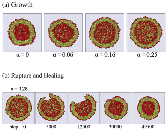
These image come from Lin, C.-M., Wu, D. T., Tsao, H.-K. & Sheng, Y.-J. Membrane properties of swollen vesicles: growth, rupture, and fusion. Soft Matter 8, 6139 (2012).
This image comes from Deserno, M. Mesoscopic Membrane Physics: Concepts, Simulations, and Selected Applications. Macromol. Rapid Commun. 30, 752–771 (2009).
My MD simulations
I combined the MD simulation method from Lin et al. and the coarse-grained lipid structure from Deserno et al.
Here is my code.
Dissipative Particle Dynamics (DPD)
- mesoscopic simulation method
- link between simulation parameters and Flory-Huggins $\chi$-parameters
- DPD fluid has quadratic equation of state
- simulate fragments to derive $\chi$-parameters
- possible problem with timescale separation between particle diffusion and momentum diffusion (viscosity)
- soft condensed matter systems have relevant length scale between atomistic and macroscopic scales
- polymer gels have length scale set by distance between crosslinks
- simple bead and spring model predicts universal linear viscoelastic behavior
- indicates lifetimes/structures of crosslinks matters more than chemical details
- surfactant mesophases have length scale set by wavelength of fluctuations
- diverse phase behavior: lamellar structures, gels, micelles, networks
- lattice techniques not suited to branched or multiblock copolymers
- macroscopic simulations of associative liquids do not describe molecular details or hydrodynamic interactions
- [11, 12] Hoogerbrugge and Koelman introduced dissipative particle dynamics (DPD)
- soft spheres with collision rules
- bead and spring particles to simulate polymers
- [15] Español and Warren studied fluctuation-dissipation theorem in DPD
- three forces: conservative, dissipative, random
- for statistical mechanics to correspond to canonical ensemble, dissipative and random forces must satisfy a relation
- check statistical mechanical validity as a function of the time step size
- simple scaling relation, to relate model parameters to Flory-Huggins polymer theory
- can calculate solubility parameters from atomistic simulations
DPD Simulation Method
- time evolution from Newton's equations of motion
- set masses to unity
- sum forces with cutoff radius $r_c$
- set cutoff radius to unity
- conservative force, soft repulsion along line of centers
$$F_{ij}^C = \left\{ \begin{array}{c} a_{ij} \left(1 - r_{ij}\right) \hat r_{ij}, r_{ij} < 1 \\ 0, r_{ij} \ge 1 \end{array} \right.$$
- dissipative force: acts opposite relative velocity between particles
$$F_{ij}^D = - \gamma w_D \left( r_{ij} \right) \left(\hat r_{ij} \cdot \vec v_{ij} \right) \hat r_{ij}$$
- random force: to conserve momentum, should use same value of random variable for both $F_{ij}^R$ and $F_{ji}^R$
$$F_{ij}^R = \sigma w_R \left( r_{ij} \right) \theta_{ij} \hat r_{ij}$$
- $w_D$ and $w_R$ are weight functions that vanish beyond the cutoff radius $r_c$
- $\theta_{ij}$ is a random variable with Gaussian statistics
$$\left< \theta_{ij} (t) \right> = 0, \left< \theta_{ij} (t) \theta_{kl} (t^\prime) \right> = \left( \delta_{ik} \delta_{jl} + \delta_{il} \delta_{jk} \right) \delta (t - t^\prime)$$
- both dissipative and random forces act along line of centers, conserve linear and angular momentum
- independent random function for each pair (emphasized, see note above) of particles
- review fluctuation-dissipation theorem
$$w_D(r) = \left( w_R(r)\right)^2 = (1 - r)^2 r < 1, \sigma^2 = 2 \gamma k_B T$$
- chose $w_R(r)$ same functional form as conservative force
- Fokker-Planck equation governs time evolution of probability distribution
$$\frac{\partial \rho}{\partial t} = \mathcal{L}^C \rho + \mathcal{L}^D \rho$$
- $\mathcal{L}^C$ the Liouville operator of Hamiltonian system with conserved forces $F^C$
- $\mathcal{L}^D$ contains dissipative and noise terms
- without dissipation and noise, Gibbs-Boltzmann distribution a solution of $\partial \rho / \partial t = \mathcal{L}^C \rho = 0$
- with dissipation and noise, must still satisfy Gibbs-Boltzmann distribution $\mathcal{L}^D \rho = 0$
- review why dissipation and noise should not violate Gibbs-Boltzmann
- if new distribution matches Gibbs-Boltzmann, can use standard thermodynamic relations
- NVT molecular dynamics can simulate Hamiltonian system in canonical ensemble, why DPD?
- can view DPD as novel thermostat
- and DPD preserves hydrodynamics
- annealing defects in ordered mesophases
- dynamic density functional theory or Monte Carlo methods do not preserve hydrodynamics
- soft interaction potential another advantage over simulations with Lennard-Jones atoms
- allows much larger time step
- to obtain soft potentials, average molecular field over rapid atomic motions
- does not diverge at $r = 0$ and lacks characteristic minimum of LJ potential
- needs complicated integrations, similar to virial coefficients in low density expansion
- so no analytical expression for effective interaction potential
- neglects correlation in local density fluctuations
- Groot and Warren suggest a pragmatic alternative
- top down rather than bottom up, match thermodynamics
- set $k_B T = 1$ specifies time, as rms velocity $\sqrt{3}$ from MB distribution
- how to choose time step
- compromise between fast simulation and equilibrium condition
- monitor system temperature
- no statistical difference between uniform and Gaussian random numbers
- uniform random numbers take less CPU time than Gaussian numbers
- artificial temperature increase influences time step choice
- compared to Euler, Verlet with acceleration term gives 50 fold improvement (both needed)
- equilibration time decreases as noise/dissipation amplitude increases
- temperature increases with noise amplitude
- how to choose repulsion parameter
- must choose $a$ to describe fluctuations in the liquid, related to compressibility
- analogous to Weeks-Chandler-Anderson perturbation theory of liquids
$$\kappa^{-1} = \frac{1}{n k_B T \kappa_T} = \beta \left. \frac{\partial \rho}{\partial n} \right|_T$$
- $\kappa_T$ is the isothermal compressibility
- obtain pressure via virial theorem as
$$p = \rho k_B T + \frac{1}{3V} \left< \sum_{j > i} \left( \vec r_i - \vec r_j \right) \cdot \vec f_i \right>$$
- radial distribution function: how density varies with respect to distance from particle
- surface tension: integral over stress across an interface
- excess pressure scales linearly with repulsion parameter, proportional to $\rho^2$
- CPU time increases with square of density
- choose lowest density that satisfies scaling relation
- $a = 75 k_B T / \rho$
- soft repulsion, apparent absence of $\rho^3$ term at high densities
- cannot produce liquid-vapor coexistence
- review details
- steep repulsion at small $r$ spoils temperature control
$$\frac{F}{k_B T} = \frac{\phi_A}{N_A} \ln \phi_A + \frac{\phi_B}{N_B} \ln \phi_B + \chi \phi_A \phi_B$$
- do not favor contact $\chi > 0$
-
- to advance state
- simple Euler algorithm
- must include a factor of $\Delta t^{-1/2}$ in random force
- integrate stochastic differential equations
- interpret random force as Wiener process
- let random force have zero mean and variance $\sigma^2$
- if variance has no dependence on time step, unphysical behavior
- mean square value of time integral proportional to the square distance i.e. to the time
- mean diffusion must have finite value independent of integration step size
- spread of random force increases as we subdivide the time interval
- modified version of velocity Verlet algorithm
- prediction for new velocity corrected in last step
- force updated once per iteration
- temperature updated after last step
- stochasticity makes order of algorithm unclear
- lambda = 1/2
Models
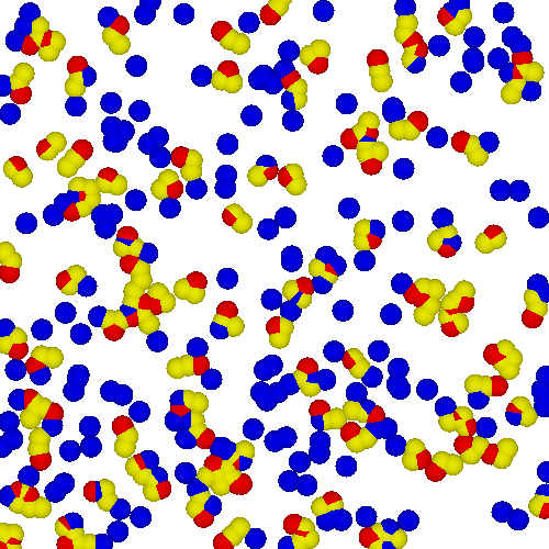
Per molecule, we have two nonpolar monomers and one polar monomer - this approximates the aspect ratios of the lipid constituents, important to the morphologies achieved by the lipids. Furthermore, the size of the head group compared to the size of the two tail groups can dramatically influence the equilibrium phase behavior.
- Monomer size/penetration: Weeks-Chandler-Andersen potential (WCA) $$V_{\rm rep}(r, b) = \left\{ \begin{eqnarray} 4 \epsilon \left[ \left( \frac{b}{r} \right)^{12} - \left( \frac{b}{r} \right)^6 + \frac{1}{4} \right] &,& \,\,\,\, r \le r_c \\ 0 &,& \,\,\,\, r > r_c \end{eqnarray} \right.$$
- Bonds between connected monomers in lipids: Finite extensible nonlinear elastic (FENE) $$V_{\rm bond} = - \frac{1}{2} k_{\rm bond} r_\infty^2 \ln \left[ 1 - \left( \frac{r}{r_\infty} \right)^2 \right]$$
- Bending rigidity of lipid: harmonic spring $$V_{\rm bend} = \frac{1}{2} k_{\rm bend} (r - 4 \sigma)^2$$
- Interaction between nonpolar tail groups: Need to be careful with this one in order to achieve fluid properties (if interaction too short range, then only achieve gas and gel phases)$$V_{\rm attr}(r) = \left\{ \begin{eqnarray} - \epsilon &,& \,\,\,\, r < r_c \\ - \epsilon \cos^2 \frac{\pi \left( r - r_c \right)}{2 w_c} &,& \,\,\,\, r_c \le r \le r_c + w_c \\ 0 &,& \,\,\,\, r > r_c + w_c \end{eqnarray} \right.$$
Questions
I seek to understand membrane rupture. I will take this strategy
- First model vesicles.
- Next, add inert spheres inside/outside the vesicles.
- At what ramp rates/concentrations do the vesicles implode?
- How big are holes that form?
Approach
- 1. To find equilibrium starting configurations, identify local minima in energy landscapes, using material from the search and optimization sections. To decrease time required to evaluate energy of system, truncate range of potential.
- 2. To obtain some dynamical information, solve Newton's equations directly. Use an algorithm such as the Verlet algorithm. This will use information from the random systems and partial differential equations section.
- 3. I will compete this against a package for molecular dynamics simulations, an MD environment called ESPResSo (Extensible Simulation Package for RESearch on SOft Matter), developed for simulation of soft matter systems with electrostatic interactions. I downloaded and complied Tcl/Tk and ran a few Espresso tutorials. For visualization, I have downloaded and used plugins to export Espresso output into VMD (Visual Molecular Dynamics).
Data structure
- from Numerical Simulation in Molecular Dynamics: Numerics, Algorithms, Parallelization, Applications
- by Michael Griebel, Stephan Knapek, and Gerhard Zumbusch
- our DPD model has short-range interactions, need only consider neighbors
- in 2D, a 4N-dimensional phase space
- assume a square or rectangular simulation domain
- periodic boundary conditions (PBC) to compensate for limited size of simulation domain
- for Lennard-Jones potential, cutoff radius typically about $2.5 \sigma$
- in our case, we define cutoff radius in DPD interactions
Linked Cell Method
- split physical simulation domain into uniform subdomains
- choose cell size equal to or greater than cutoff radius
- then particles in a cell interact only with particles in the cell and in neighboring cells
- compute force on particle as sum over particles within sum over neighboring cells
- complexity reduced from $\mathcal{O}\left(N^2 \right)$ to $\mathcal{O}\left(N \right)$
- need appropriate data structures
- in 2D, assign indices $\left(c_x, c_y \right)$ to cells; each cell has 8 neighbors
- particles located in one cell stored in a linked list associated with the cell
- need a dynamic data structure for the particles of each cell
- [559, 560] linked list references
- each element consists of the particle and a pointer next to the next element of the list
- remove from one list, and insert to the beginning of another list
- i->next = *root_list;
- i is a pointer to the inserted particle
- sets the next pointer to point to the current first particle
- *root_list = i;
- i is a pointer to the inserted particle
- sets the pointer to the new first particle i
- with removal operation, must change next of previous element
- in a simple list, no direct way to find previous element
- easy to implement if pointers in both directions
- if inflow or outflow conditions, should remove element and perhaps release memory
- with PBC, need not worry can just move elements from one list to another
- cell represented as root pointer of the list
- size and position of cell determined from global parameters
- define vector grid of cells of type cell (root_list pointers)
- take 2d and vectorize
- i->p points to the first particle in the linked list
- i = i->next to advance from one element to the next
- outer loop over all cells, inner loop over all particles
- can put the simulation into the idle loop
- decided to make one structure, with an integer that flags the molecule as either a lipid or a water, so the linked list just points to a single structure
- had trouble making an array of pointers
- fixed by using the ampersand operator
- figured out how to change the view angle in OpenGL
- can use the glOrtho to do 3d slices through the 3d volume as soon as I set that up
- finished initialization of the particles
- GOT TO FIGURE OUT pointers and linked lists!
- remember to put ; after structure definitions!
- got the insert function working! woo hoo!
- decided to make a doubly linked list in order to facilitate the remove function
- memory allocation problems..
- got the linked list working! :) woo hoo!
Implementation
- linked cell method https://www10.cs.fau.de/Teaching/Courses/SS2009/AlgCSE/presentation_aprelkin.pdf
- linked list associated with each cell
- cell represented by root pointer to the cell
- grid cells stored in a vector
- can decrease number of forces by summing over pairs/forces rather than particles
- C tutorials by Alex Allain
- linked list: http://www.cprogramming.com/tutorial/c/lesson15.html
Rendering
- thought to use VMD
- realized just plotting spheres, did not need all the complexity
- decided to practice with OpenGL
- found a tutorial here http://www.swiftless.com/tutorials/opengl/collision.html
- had to remember how to compile the openGL code on Mac
- openGL has a stack of matrices
- push copies the top matrix and adds it to the top of the stack
- pop deletes the top matrix from the top of the stack
- initially, each of the stacks contains one matrix, the identity
- on a Mac, need to include #include header file
- to compile need to include framework flags
- gcc gl_spheres.c -o gl_spheres -framework OpenGL -framework GLUT
- can make a bunch of spheres by doing
glPushMatrix();

		position = (float)x / 20;

		glTranslatef(-position, position, -position);

		glutSolidSphere(0.05, 40, 40);

		glPopMatrix();
- tried to make spheres at random locations, will need randomness in force expression
- decided to write LFSR in c, had written in python for a previous assignment
- learned about number representations in c
- the "0b" prefix did not work right away
- read about hexadecimal representation, starts with "0x"
- from http://www.cprogramming.com/tutorial/bitwise_operators.html
- the byte is lowest level at which we can access data
- most significant bit to the left
- need to be careful about storage, can end up with modular arithmetic
- bitwise AND: ampersand &, can use to find the bit in the nth position
- can use bitwise leftshift to generate the mask
- bitwise OR: line |
- bitwise complement: ~
- bitwise XOR: ^
- tried the bitwise complement and encountered twos complement
- struggled with adding numbers together - e.g., tried to add 1 and 8 to make 9, and instead got 32776, I think it has something to do with adding the numbers as binary variables rather than as integers, and with the signed integers, twos complement thing.
- NO! just had to do with initial value of variable when declared was 2^15..!?
- ran into trouble passing variables into main - seemed fixed after I put the function arguments into main rather than passing them in (function main takes zero or two arguments)
- Charles taught me about textmate, a convenient editor that lets me run the code without switching back and forth between the editor and the terminal to compile then run the code also saved at the same time
- finished implementation of the LFSR - can treat numbers as binaries and act on them directly.
- wait a sec - worked with M = 4, but did not immediately work with M = 5
- was indexing in the wrong direction, and had gotten lucky because before had worked because M = 4 takes the first and last one, whereas M = 5 the first and second to last, so the second to last didn't catch the first and all the bits got pushed off the register. note that all the indices in the register have the first bit in the tap, otherwise 1 would not cycle back
- M = 23 somehow looked much worse than M = 24
- no made a mistake (assigned 2 and 3 to 0 and 1), but still looked random
- great openGL tutorials at http://www.swiftless.com/tutorials/opengl/color.html
- just needed glEnable(GL_COLOR_MATERIAL) and then could set color with glColor
- decided to start in 2d and then graduate to 3d
- as not to waste too much time with the rendering etc.