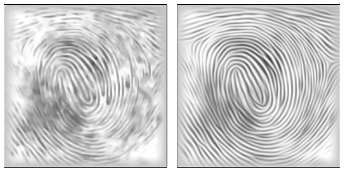
Shows space-variant coherence-enhancing diffusion used to enhance fingerprint image.
I will study methods of simulating diffusion, and attempt to apply them to visualize graph data. More specifically, I'm interested in simulating space-variant diffusion, in which the degree of diffusivity changes depending on the location.
Methods for simulating space-variant diffusion were originally developed by the image processing community to denoise images in a way that preserved (or even uncovered) structure and important details.
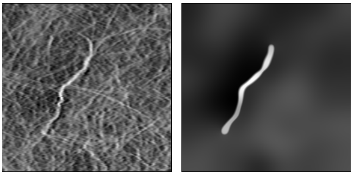
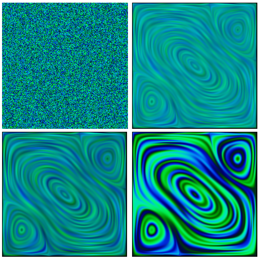
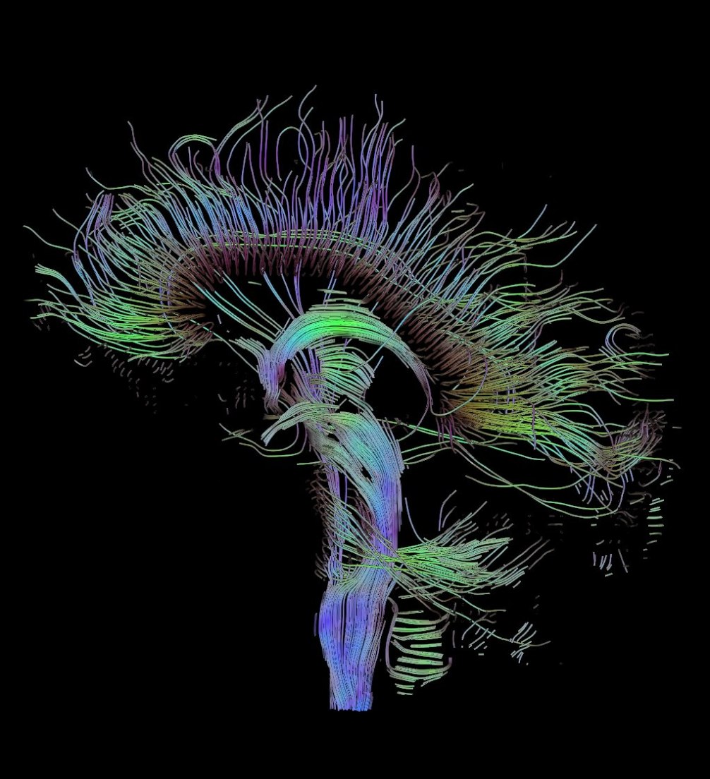
These methods have subsequently been helpful for imaging very different types of data, including vector fields and brain tissue.
Graph data shares interesting properties with these datasets.
Certain graphs such as transportation networks express information about flow, like vector fields.
When visualized, graphs contain geometric structure which can resemble biological tissue.
Therefore, I wanted to see whether methods of space-variant diffusion could be used for graph visualization.
To implement space-invariant diffusion on an image, you solve the heat equation over each pixel, where the local gradients are found by comparing each pixel's intensity with that of its neighbors:
$${\delta u \over \delta t} = div \Big(\nabla u \Big) $$
Where $u$ is the image. This equation serves to move each pixel towards the average of its neighbors.
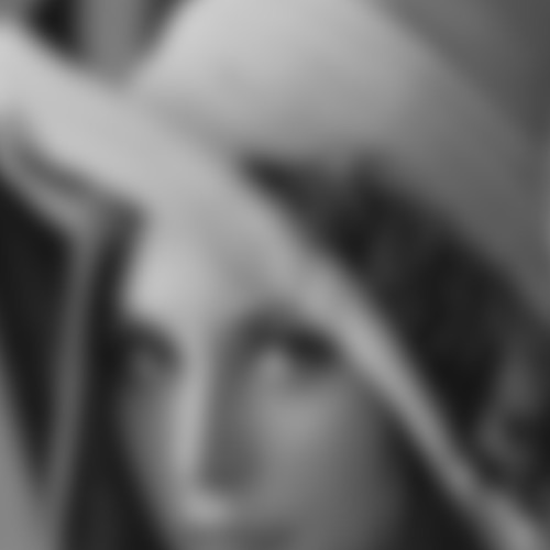
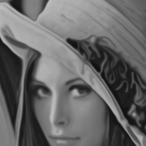
Just to establish a baseline, here is what space-invariant diffusion looks like on the Lena image:
As you can see, both noise and structure are eliminated as the diffusion proceeds.
Perona and Malik developed a model of space-invariant diffusion that reduces noise and enhances edges by scaling the diffusivity at each pixel according to how much change is detected in the neighborhood of that pixel. The continuous form of their model can be stated like this:
$${\delta u \over \delta t} = div \Big(g(| \nabla u |) \nabla u \Big) $$
Where $g$ is a function chosen so that diffusion is maximal where the gradient is small (within uniform regions), and minimal where the gradient is large (against edges).
$$g(x) = exp \Big(-(x / \kappa)^2 \Big) $$
Here, $\kappa$ is the gradient threshold parameter, which tunes the sensitivity to noise. The higher $\kappa$ is, the larger the gradients must be before being attributed to edges as opposed to noise.
Perona-Malik diffusion can be discretized like this:
$$ u_{t+1}(s) = u_{t}(s) + { \lambda \over |\eta_{s}| } \displaystyle\sum_{p \in \eta_{s}} g(|\nabla u_{s,p}|) \nabla u_{s,p} $$
Here, $s$ is a particular pixel in the image, $\lambda \in (0,1]$ is the rate of diffusion, and $\eta \in \{N, S, E, W\}$ refers to the four directions of diffusion in the image.
Whereas $\nabla$ in the continuous form represents the gradient of the image, in the discretization it represents the difference between the image at a point $s$, and the image at the pixels adjacent (in the $N, S, E, W$ directions) to $s$.
$$ \nabla u_{s,p} = u_{t}(p) - u_{t}(s) $$
Here are still images of space-invariant and Perona-Malik diffusion after 50 iterations:
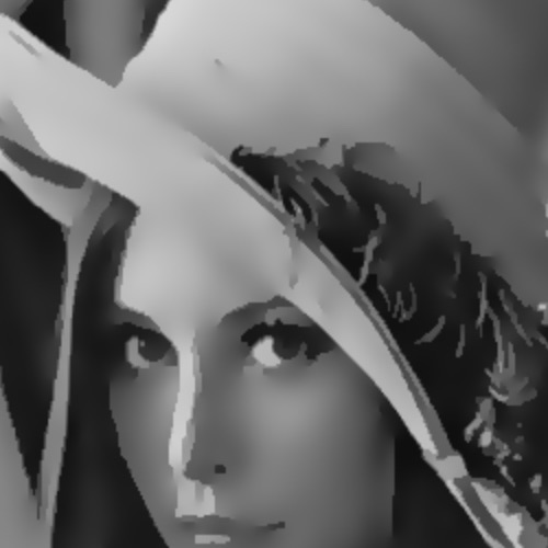
As can be observed in the above diagrams, while Perona-Malik is clearly superior to isotropic diffusion in terms of preserving structure, there is still a lot of noise. For example, in the Lena image, while diffusion indeed stops at the edge of her hat, the outline of her hat remains very noisy. And in the vector field, Perona-Malik almost completely degrades to isotropic diffusion when we go off the axes of the discretization.
These issues motivated the development of anisotropic diffusion. Isotropic diffusion uses a constant scalar diffusivity, Perona-Malik uses a spatially varying scalar diffusivity, and anisotropic diffusion uses a spatially varying tensor diffusivity. The reason this will solve the problems I just noted is that the tensor will allow us to actually change the direction of diffusion, depending on the local structure. So, while Perona-Malik only requires that we stop smoothing when we get to an edge, anisotropic diffusion will allow us to smooth with small elongated kernels along edges, and Gaussian kernels in uniform regions.
The diffusion tensor is based on the structure tensor of the image. The structure tensor captures the predominant directions of the gradient around a point, and the degree to which those directions are coherent. In contrast, Perona-Malik's discretization averages the gradient around a point.
Anisotropic diffusion is described by the following equation:
$${\delta u \over \delta t} = \nabla \cdot (D \nabla u) $$
$$D = \begin{pmatrix} D_{11} & D_{12} \\ D_{12} & D_{22} \\ \end{pmatrix}$$
Here, $u$ is the image, $t$ is the diffusion time, and $D$ is the diffusion tensor.
The diffusion tensor characterizes the local magnitude, orientation, and anisotropy of the diffusion at any point within the image. It is derived from the structure tensor $J$ of the image. Specifically:
$$J_{\rho}(\nabla u_{\sigma}) = G_{\rho} * ( \nabla u_{\sigma} \nabla u_{\sigma}^T )$$
$$J_{\rho} = \begin{pmatrix} J_{11} & J_{12} \\ J_{12} & J_{22} \\ \end{pmatrix}$$
$G_{\rho}$ is a Gaussian with standard deviation $\rho$, and $u_{\sigma}$ is the image data after convolution with a Gaussian. The eigenvectors of the structure tensor express the local orientation of the gradient, and its corresponding eigenvalues express the degree to which the gradient aligns with them.
The eigenvalues $\mu_{1}, \mu_{2}$ of $J$ are:
$$\mu_{1} = {\frac{1}{2}} \Big( J_{11} + J_{22} + \sqrt{(J_{11} - J_{22})^2 + 4J_{12}^2} \Big)$$
$$\mu_{2} = {\frac{1}{2}} \Big( J_{11} + J_{22} - \sqrt{(J_{11} - J_{22})^2 + 4J_{12}^2} \Big)$$
The eigenvectors of $D$ are:
$$v_{1} = 2 J_{12}$$
$$v_{2} = J_{22} - J_{11} + \sqrt{(J_{11} - J_{22})^2 + 4J_{12}^2}$$
In constructing the diffusion tensor, suppose we want to enhance edges. Then we can choose the eigenvalues ($\lambda_{1}, \lambda_{2}$) of the diffusion tensor such that we reduce diffusivity in the direction perpendicular to the gradient as $\mu_{1}$ (the strength of the gradient) increases.
$$\lambda_{1}(\mu_{1}) = 1 - exp \Big( {-C_{m} \over (s / \lambda)^m} \Big)$$
$$\lambda_{2} = 1$$
Now we can construct the diffusion tensor $D$
$$D_{i,j} = \displaystyle\sum_{n = 1..2} \lambda_{n} v_{ni} v_{nj}$$
We discretize $\delta u \over \delta t$ using explicit finite difference approximation. The structure of the approximation is:
$${{u_{i,j}^{k + 1} - u_{i,j}^k} \over \tau} = A_{i,j}^k * u_{i,j}^k$$
$$u_{i,j}^{k + 1} = \tau \Big(A_{i,j}^k * u_{i,j}^k \Big) + u_{i,j}^k$$
Here, $\tau$ is the time step, and $u_{i,j}^k$ represents the image at pixel $(i,j)$ time $k\tau$. $A_{i,j}^k * u_{i,j}^k$ is the discretization of $\nabla \cdot (D \nabla u)$.
Specifically:
$$\nabla \cdot (D \nabla u) = \delta_{x} j_{1} + \delta_{y} j_{2}$$
$$j_{1} = D_{11}(\delta_{x} u) + D_{12}(\delta_{y} u)$$
$$j_{2} = D_{12}(\delta_{x} u) + D_{22}(\delta_{y} u)$$
Where:
$$\delta_{y} (D_{12} (\delta_{x} u)) = {1 \over 2} \Big(D_{12(i,j + 1)} {{u_{(i + 1,j + 1)} - u_{(i - 1,j + 1)}} \over 2} - D_{12(i,j - 1)} {{u_{(i + 1,j - 1)} - u_{(i - 1,j - 1)}} \over 2} \Big)$$
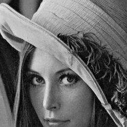
Anisotropic diffusion is best able to de-noise while preserving and even enhancing structure within the image.
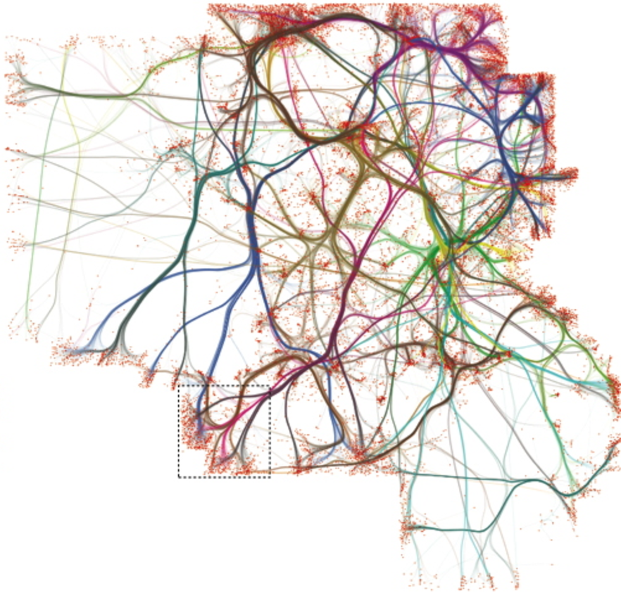
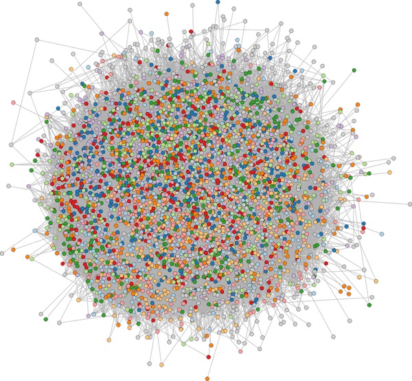
I set up a pipeline to convert a graph into a vector field. The graph consists of 5,000 nodes and ~28,000 edges. The nodes are Twitter users, and edges denote mutual followership. The nodes are colored by political ideology.
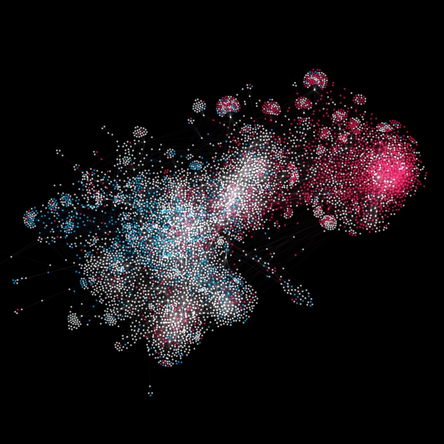
In order to convert this graph into a vector field, I used the following method. First I defined a resolution for displaying my vector field: a 500x500 canvas. Then, for each edge in my graph, I traced it through my canvas. Every time the edge crossed a new pixel in my canvas, I recorded its slope in that pixel. Finally, I defined a slope for each pixel in my canvas by taking the average slope of all the edges that pass through it.
I wanted to see whether visualizing a graph this way would illuminate patterns of information diffusion that couldn’t be seen with a traditional force layout.
Why I thought this method might succeed:
Why I failed: