Chapter 9 - Finite Element Analysis
(9.1) Consider the damped wave equation $\frac{\partial^2u}{\partial t}= v^2\frac{\partial^2 u}{\partial x^2}+\gamma\frac{\partial}{\partial t}\frac{\partial^2 u}{\partial x^2}$ and take the solution domain to be the interval $[0, 1]$.
(a) Use the Galerkin method to find an approximating system of differential equations.
We assume that the solution is a sum of basis functions $\phi_i$ multiplied by coefficients $a_i$. Illustratively, $$u(x,t) = \sum_i a_i(t)\phi_i(x) \text{ . }$$
Solving the Galerkin integral, we have $$\int_0^1 R(x,t) \phi_j(x)dx = 0 \\ \int_0^1 \Big(\frac{\partial^2u}{\partial t} - v^2\frac{\partial^2 u}{\partial x^2}-\gamma\frac{\partial}{\partial t}\frac{\partial^2 u}{\partial x^2}\Big) \phi_j(x)dx = 0 $$ , substituting with the form of the solution we assumed, and regrouping $$ \int_0^1 \sum_i\Big(\frac{\partial^2 a_i\phi_i}{\partial t} - v^2\frac{\partial^2 a_i\phi_i}{\partial x^2}-\gamma\frac{\partial}{\partial t}\frac{\partial^2 a_i\phi_i}{\partial x^2}\Big) \phi_j(x)dx = 0 \\ \sum_i \frac{d a_i(t)}{dt^2}\int_0^1\phi_i(x)\phi_j(x)dx - \sum_i[v^2 a_i(t) + \gamma \frac{d a_i(t)}{dt}]\int_0^1 \frac{d^2\phi_i(x)}{dx^2}\phi_j(x)dx = 0 \\ \sum_i \frac{d a_i(t)}{dt^2}\int_0^1\phi_i(x)\phi_j(x)dx - \sum_i[v^2 a_i(t) + \gamma \frac{d a_i(t)}{dt}] \Big( \frac{d\phi_i(x)}{dx}\phi_j \Big|_0^1 - \int_0^1 \frac{d\phi_i(x)}{dx}\frac{d\phi_j(x)}{dx}dx \Big)= 0 $$
In a matrix form, we have $$ \mathbf{A}\frac{d \vec{a}(t)}{dt^2} - \gamma \mathbf{B} \frac{d \vec{a}(t)}{dt} - v^2 \mathbf{B}\vec{a} = 0$$ ,where $$\begin{align} A_{ij} &= \int_0^1\phi_i(x)\phi_j(x)dx \\ B_{ij} &= \frac{d\phi_i(x)}{dx}\phi_j \Big|_0^1 - \int_0^1 \frac{d\phi_i(x)}{dx}\frac{d\phi_j(x)}{dx}dx \end{align}$$
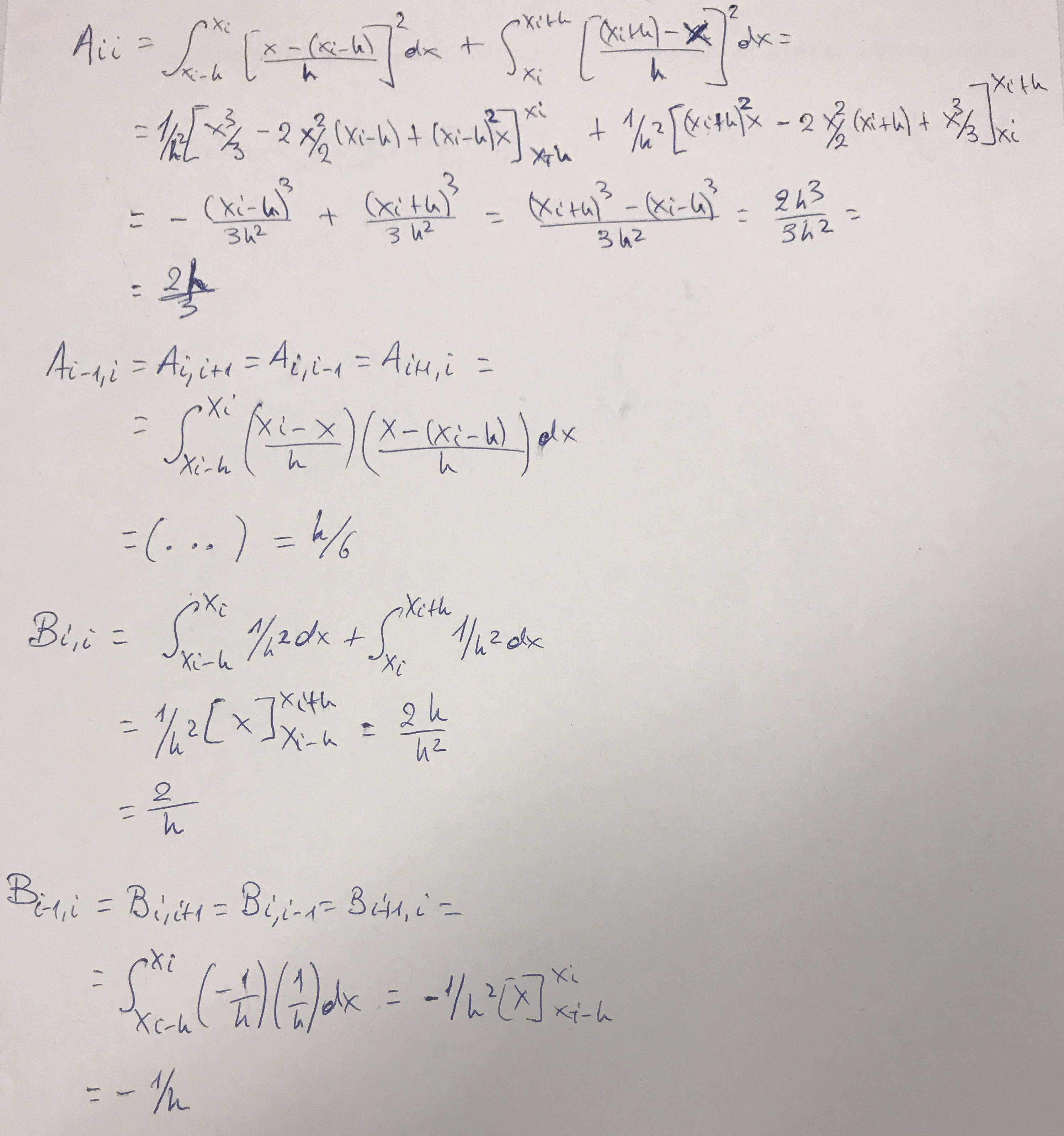
(b) Evaluate the matrix of coefficients for linear hat basis functions, using elements with a fixed size of $h$.
From Figure (9.1) and equation (9.8), we just need to find the diagonal and one-off diagonal elements of the matrices $\mathbf{A}$ and $\mathbf{B}$ (the integrals overlap only between $x_{i-1}$ and $x_{i+1}$.
(c) Now find the matrix coefficients for Hermite polynomial interpolation basis functions, once again using elements with a fixed size of $h$.
Using SymPy to compute the four basis functions in Figure 9.2 with equation 9.21
import sympy as sm
from sympy.matrices import Matrix, MatMul

x,h = sm.symbols('x h')

# First creating the matrix from equation 9.21
M = Matrix([[1,0,0,0],[0,1,0,0],[1,h,h**2,h**3],[0,1,2*h,3*h**2]])

# Inverting the matrix
M_inv = M.inv()

# Calculating the four shape functions and their derivatives
u = [[] for _ in range(4)]
du = [[] for _ in range(4)]
for i in range(4):
    u[i] = M_inv[:,i].T * Matrix([1, x, x**2, x**3])
    du[i] = sm.diff(u[i], x)
And subsequently using again SymPy to compute the integrals for the coefficients. For the $\mathbf{A}$ matrix:
from IPython.display import display, Math
sm.init_printing(use_latex='mathjax')
# For the u basis functions
Adiag = sm.integrate(u[2]*u[2], (x,0,h)) +  sm.integrate(u[0]*u[0], (x,0,h))  # Diagonal
Aoff = sm.integrate(u[0]*u[2], (x,0,h)) # Off-diagonal
display(Math('A_{u_i,u_i}'), Adiag)
display(Math('A_{u_{i-1},u_i}'), Aoff)

# For the du basis functions
Adiag = sm.integrate(u[3]*u[3], (x,0,h)) +  sm.integrate(u[1]*u[1], (x,0,h))  # Diagonal
Aoff = sm.integrate(u[1]*u[3], (x,0,h)) # Off-diagonal
display(Math('A_{\dot{u}_i,\dot{u}_i}'), Adiag)
display(Math('A_{\dot{u}_{i-1},\dot{u}_i}'), Aoff)


# And finally the cross
Adiag = sm.integrate(u[2]*u[3], (x,0,h)) +  sm.integrate(u[1]*u[2], (x,0,h))  # Diagonal
Aoff = sm.integrate(u[1]*u[2], (x,0,h)) # Off-diagonal
display(Math('A_{\dot{u}_i,u_i}'), Adiag)
display(Math('A_{\dot{u}_{i-1},u_i}'), Aoff)
And similarly for the $\mathbf{B}$ matrix:
# For the u basis functions
Bdiag = sm.integrate(du[2]*du[2], (x,0,h)) +  sm.integrate(du[0]*du[0], (x,0,h))  # Diagonal
Boff = sm.integrate(du[0]*du[2], (x,0,h)) # Off-diagonal
display(Math('B_{u_i,u_i}'), Bdiag)
display(Math('B_{u_{i-1},u_i}'), Boff)

# For the du basis functions
Bdiag = sm.integrate(du[3]*du[3], (x,0,h)) +  sm.integrate(du[1]*du[1], (x,0,h))  # Diagonal
Boff = sm.integrate(du[1]*du[3], (x,0,h)) # Off-diagonal
display(Math('B_{\dot{u}_i,\dot{u}_i}'), Bdiag)
display(Math('B_{\dot{u}_{i-1},\dot{u}_i}'), Boff)


# And finally the cross
Bdiag = sm.integrate(du[2]*du[3], (x,0,h)) +  sm.integrate(du[1]*du[2], (x,0,h))  # Diagonal
Boff = sm.integrate(du[1]*du[2], (x,0,h)) # Off-diagonal
display(Math('B_{\dot{u}_i,u_i}'), Bdiag)
display(Math('B_{\dot{u}_{i-1},u_i}'), Boff)
(9.2) Model the bending of a beam (equation 9.29) under an applied load. Use Hermite polynomial interpolation, and boundary conditions fixing the displacement and slope at one end.