Implementation and working notes of Final Project
A] Initial final project direction: Iterative parameter fitting and model selection.
Initially I wanted to explore function fitting using neural networks, in order to get a sense of a data driven parameter estimation. The ideas was to train a neural network fit the parameters of a given function family into a set of datapoints, with aim to use the same network architecture for model selection.
To explain the last sentence, let's assume that we have a function of the form $f(\vec{x})=\sum_i m_iu_i(\vec{x})$, where $u_i$ is a diverse set of functions. For example, $$f(x) = m_1[\alpha sin(\beta x)] + m_2 \log(x) + m_3 x^2 \text{ . }$$
The neural network would have to learn the parameters $m_i$, which is essential a model selection for the underlying function. Of course, this approach relies heavily on knowledge about the domain of the dataset, which will be used to form the set of functions $u_i$ that the network would have to select for.
Investigating function approximation with neural nets
%matplotlib inline
import numpy as np
import matplotlib.pyplot as plt
import seaborn as sns
sns.set_style('white')
sns.set_context('notebook')
import keras
import keras.backend as K
from keras.models import Sequential
from keras.layers import Dense, Activation
from keras.callbacks import EarlyStopping
x = np.arange(-10, 10, 0.01)
y1 = 2*x**2 + 3
f1 = lambda x: 2*x**2 + 3
x_train = np.random.choice(x, size=1000)
y_train = f1(x_train)
def train_simple_neural_network(x_train, y_train, x_test, y_test, n_neurons=2, epochs=1000, batch_size=50):
    model = Sequential()
    model.add(Dense(n_neurons, input_shape=(1,)))
    model.add(Activation('sigmoid'))
    model.add(Dense(1,use_bias=False))
    model.add(Activation('linear'))

    model.compile(loss='mse',
                  optimizer='sgd')

    history = model.fit(x_train, y_train,
                    batch_size=batch_size,
                    epochs=epochs,
                    verbose=0,
                    validation_split=0,
                    callbacks=[EarlyStopping(patience=20, min_delta=.001, monitor='loss')])

    y_pred = model.predict(x_test, batch_size=50, verbose=1)
    error = model.evaluate(x_test, y_test, batch_size=50, verbose=1)

    return y_pred, model.count_params(), error
plt.scatter(x, y1, label='Function')
for n in [1, 2, 5, 10]:
    y_pred, params, error = train_simple_neural_network(x_train, y_train, x, y1, n_neurons=n)
    plt.scatter(x, y_pred, label='%d Neurons, %d params, %.3f Error' % (n, params, error))
plt.legend()
plt.show()

plt.scatter(x, y1, label='Function')
for n in [10, 20, 50, 100]:
    y_pred, params, error = train_simple_neural_network(x_train, y_train, x, y1, n_neurons=n)
    plt.scatter(x, y_pred, label='%d Neurons, %d params, %.3f Error' % (n, params, error))
plt.legend()
plt.show()

def train_univ_neural_network(x_train, y_train, x_test, y_test, n_neurons=None):
    if n_neurons==None:
        n_neurons=[]
    model = Sequential()
    model.add(Dense(n_neurons[0], input_shape=(1,)))
    model.add(Activation('sigmoid'))
    model.add(Dense(n_neurons[1], input_shape=(1,)))
    model.add(Activation('sigmoid'))
    model.add(Dense(1,use_bias=False))
    model.add(Activation('linear'))

    model.compile(loss='mse',
                  optimizer='sgd')

    history = model.fit(x_train, y_train,
                    batch_size=100,
                    epochs=1000,
                    verbose=0,
                    validation_split=0,
                    callbacks=[EarlyStopping(patience=20, min_delta=.001, monitor='loss')])

    y_pred = model.predict(x_test, batch_size=50, verbose=1)
    error = model.evaluate(x_test, y_test, batch_size=50, verbose=1)

    return y_pred, model.count_params(), error
plt.scatter(x, y1, label='Function')
for n in [1, 2, 5, 10]:
    y_pred, params, error = train_univ_neural_network(x_train, y_train, x, y1, n_neurons=[n,n])
    plt.scatter(x, y_pred, label='%d Neurons, %d params, %.3f Error' % (n, params, error))
plt.legend()
plt.show()

plt.scatter(x, y1, label='Function')
for n in [10, 20, 50, 100]:
    y_pred, params, error = train_univ_neural_network(x_train, y_train, x, y1, n_neurons=[n, n//2])
    plt.scatter(x, y_pred, label='%d Neurons, %d params, %.3f Error' % (n, params, error))
plt.legend()
plt.show()

x = np.arange(-2.5, 2.5, 0.001)
y3 = np.sin(2*x**2 + 3)
f3 = lambda x: np.sin(2*x**2 + 3)
x_train3 = np.random.choice(x, size=5000)
y_train3 = f3(x_train3)
plt.scatter(x, y3, label='Function')
plt.xlim([-2.5, 2.5])
for n in [1, 2, 5, 10]:
    y_pred, params, error = train_simple_neural_network(x_train3, y_train3, x, y3, n_neurons=n, batch_size=100)
    plt.scatter(x, y_pred, label='%d Neurons, %d params, %.3f Error' % (n, params, error))
plt.legend()
plt.show()

def train_deep_neural_network(x_train, y_train, x_test, y_test, n_neurons=None, activation='sigmoid'):
    if n_neurons==None:
        n_neurons=[]
    model = Sequential()
    for i in n_neurons:
        model.add(Dense(i, input_shape=(1,)))
        model.add(Activation(activation))
    model.add(Dense(1,use_bias=False))
    model.add(Activation('linear'))

    model.compile(loss='mse',
                  optimizer='sgd')

    history = model.fit(x_train, y_train,
                    batch_size=100,
                    epochs=1000,
                    verbose=0,
                    validation_split=0,
                    callbacks=[EarlyStopping(patience=20, min_delta=.001, monitor='loss')])

    y_pred = model.predict(x_test, batch_size=50, verbose=1)
    error = model.evaluate(x_test, y_test, batch_size=50, verbose=1)

    return y_pred, model.count_params(), error
plt.scatter(x, y3, label='Function')
plt.xlim([-2.5, 2.5])
for act in ['relu', 'sigmoid', 'tanh', 'linear']:
    n = [10,10,10]
    y_pred, params, error = train_deep_neural_network(x_train3, y_train3, x, y3, n_neurons=n, activation=act)
    plt.scatter(x, y_pred, label=act)
plt.legend()
plt.show()

As you can see, there is a very subtle relationship between the neural network perfomance, and hyperparameters such as number of layers, number of neurons and activation function.
Difference between NN with and without prior for the model
x_vis = np.arange(-5., 5., .01)
y_vis = f3(x_vis)
data  = []
for lay in [1, 2, 3]:
    n = [10 for _ in range(lay)]
    y_pred, params, error = train_deep_neural_network(x_train3, y_train3, x_vis, y_vis, n_neurons=n, activation='tanh')
    data.append({'y_pred':y_pred, 'label': '%d Layers' % len(n)})
plt.plot(x_vis, y_vis, label='Function', color='k')
plt.xlim([-5., 5.])
plt.ylim([-1., 1.])
for d in data:
    plt.scatter(x_vis, d['y_pred'], label=d['label'])
plt.legend()
plt.show()

import keras.backend as K
from keras.models import Model
from keras.layers import Lambda, Input
def train_deep_neural_network_prior(x_train, y_train, x_test, y_test, n_neurons=None, activation='sigmoid'):
    if n_neurons==None:
        n_neurons=[]

    inp = Input(batch_shape=(None, 1))
    x = inp
    for i in n_neurons:
        x = Dense(i, input_shape=(1,))(x)
        x = Activation(activation)(x)
    a = Dense(1, use_bias=False, activation='linear')(x)
    b = Dense(1, use_bias=False, activation='linear')(x)
    c = Dense(1, use_bias=False, activation='linear')(x)

    def model_function(args):
        a, b, c, inp = args
        return a*K.sin(b*K.square(inp) + c)

    out = Lambda(model_function)([a, b, c, inp])

    model = Model(inp, out)

    params = Model(inp, [a, b, c])

    model.compile(loss='mse',
                  optimizer='sgd')

    history = model.fit(x_train, y_train,
                    batch_size=100,
                    epochs=1000,
                    verbose=0,
                    validation_split=0.2,
                    callbacks=[EarlyStopping(patience=20, min_delta=.001, monitor='loss')])

    y_pred = model.predict(x_test, batch_size=50, verbose=1)
    error = model.evaluate(x_test, y_test, batch_size=50, verbose=1)

    return y_pred, model.count_params(), error, history, params
x_vis = np.arange(-5.,5.,.01)
y_vis = f3(x_vis)
n = [10]
y_pred, params, error, history, param_model = train_deep_neural_network_prior(x_train3, y_train3,
                                                                 x_vis, y_vis, n_neurons=n, activation='relu')
a_v = []
b_v = []
c_v = []
for i in x_vis:
    a,b,c = param_model.predict(np.asarray([i]))
    a_v.append(a.squeeze())
    b_v.append(b.squeeze())
    c_v.append(c.squeeze())
plt.figure()
plt.title('a*sin(b*x^2 + c)')
plt.plot(x_vis, a_v, label='a')
plt.plot(x_vis, b_v, label='b')
plt.plot(x_vis, c_v, label='c')
plt.legend()
plt.show()

plt.figure()
plt.plot(x_vis, y_vis, label='Function', color='k')
plt.xlim([-5., 5.])
plt.ylim([-1., 1.])
plt.scatter(x_vis, y_pred, label='NN with Prior')
plt.legend()
plt.show()

B] Final Project: Predicting (pseudo-)randomness
Introduction
It is impossible to predict the output of a true random process, but what about a pseudo random number generator? A good implementation of a pseudo-random number generator (PRG) produces bits that are actually indistinguishable from a true random source, and its statistically properties are rigorously tested. Yet, in all cases, the output is produced by a deterministic process, programmed to generate an extremely long (you guessed well, longer than the age of the universe) sequence of bits before looping back to the start.
The purpose of this work, which is inspired by the very last problem set question of this course, is to thoroughly investigate whether (deep) neural networks can learn the underlying generating process, when given a sufficiently long run of bits from a PRG as a training set. As a test-case, I will use the Linear Feedback Shift Register PRGs that we talked about at the second week, since they provide an seemingly easy task (addition of two or four bits) for a neural network to reverse engineer.
The project is structured as follows; Initially, I will expand on previous excersice, and use several deep feed-forward neural networks. I will do a manual hyper-parameter optimization run, to find the dependencies between network architectures and the LFSR. I will continue with a selection of recurrent neural networks to show their limitations in capturing simple operations between datapoints in sequence data. Finally, to overcome the limitations of RNNs, I will try to implement a Neural Programmer, which is a novel architecture capable to learn quickly simple mathematical (or logical) operations needed to produce an output from an set or sequence of inputs.
Setting up the LFSRs
# Imports
%matplotlib inline
import numpy as np
import matplotlib.pyplot as plt
import seaborn as sns
sns.set_style('white')
sns.set_context('notebook')

from sklearn.model_selection import train_test_split
import keras
import keras.backend as K
from keras.models import Model
from keras.layers import Dense, Activation, Input
from keras.callbacks import EarlyStopping
def dectobin(dec, bits):
    binary = [int(x) for x in bin(dec)[2:]]
    return np.hstack((np.zeros(bits-len(binary), dtype=int), binary ))

# Build PRG functions
class LFSR():
    def __init__(self, xnor_bits: list, seed: int = None):
        self.xnor_bits = xnor_bits
        self.tap = max(xnor_bits)

        if seed:
            self.state = dectobin(seed, self.tap).tolist()
        else:
            self.state = np.random.randint(2, size=self.tap).tolist()

    def step(self):
        next_bit = sum([self.state[i-1] for i in self.xnor_bits]) % 2
        self.state = self.state[1:] + [next_bit]
        return next_bit

    def run_seq(self, length: int):
        return [self.step() for _ in range(length)]

    def run_gen(self):
        while 1:
            yield self.step()
Having an implementation for a generic LFSR, I consulted the table of Maximal Length Taps in order to implement four examples of LFSR PRGs that I will use for this project. To verify the implementation, but also to visually understand the properties of the LFSRs, I visualized them as 2D images.
# 4-tap
lfsr_4 = LFSR([1, 4], 5)
lfsr_4_seq = lfsr_4.run_seq(length=10000)
lfsr_4_img = np.asarray(lfsr_4_seq).reshape((100,100))

# 8-tap
lfsr_8 = LFSR([2, 3, 4, 8], 5)
lfsr_8_seq = lfsr_8.run_seq(length=10000)
lfsr_8_img = np.asarray(lfsr_8_seq).reshape((100,100))

# 23-tap
lfsr_23 = LFSR([5, 23], 5)
lfsr_23_seq = lfsr_23.run_seq(length=10000)
lfsr_23_img = np.asarray(lfsr_23_seq).reshape((100,100))

# 85-tap
lfsr_85 = LFSR([85,84,57,53], 5)
lfsr_85_seq = lfsr_85.run_seq(length=10000)
lfsr_85_img = np.asarray(lfsr_85_seq).reshape((100,100))

f, axarr = plt.subplots(2, 2)
axarr[0, 0].imshow(lfsr_4_img)
axarr[0, 0].set_title('LFSR 4-tap')
axarr[0, 1].imshow(lfsr_8_img)
axarr[0, 1].set_title('LFSR 8-tap')
axarr[1, 0].imshow(lfsr_23_img)
axarr[1, 0].set_title('LFSR 23-tap')
axarr[1, 1].imshow(lfsr_85_img)
axarr[1, 1].set_title('LFSR 85-tap')
f.subplots_adjust(hspace=0.3)
f.set_size_inches(12,12)
plt.show()

# Prepare datasets
def chunks(l, n):
    for i in range(0, len(l)-n):
        yield l[i:i + n]
def generate_dataset(sequence, window, test_size=.2, net='feed_forward'):
    data = list(chunks(sequence, window+1))
    x_data = np.array([d[:window] for d in data])
    y_data = np.array([d[window] for d in data])

    if net=='feed_forward':
        # Dataset for the feed forward
        x_train, x_valid, y_train, y_valid = train_test_split(x_data, y_data, test_size=.2, stratify=y_data)
        return x_train, x_valid, y_train, y_valid
    elif net=='recurrent':
        # Dataset for the recurrent
        x_train, x_valid, y_train, y_valid = train_test_split(x_data, y_data, test_size=.2, stratify=y_data)
        return x_train.reshape((-1,window,1)), x_valid.reshape((-1,window,1)), y_train, y_valid
    else:
        # Dataset for the autoencoder
        x_train, x_valid = train_test_split(x_data, test_size=.2)
        return x_train, x_valid
Setting up Feed-Forward Network
def train_feed_forward(x_train, y_train, x_test, y_test, n_neurons: list=None, activation='sigmoid', return_model=False):

    inp = Input(batch_shape=(None, x_train.shape[1]))
    x = inp
    for i in n_neurons:
        x = Dense(i)(x)
        x = Activation(activation)(x)

    out = Dense(1,use_bias=False, activation='sigmoid')(x)

    model = Model(inp, out)

    model.compile(loss='binary_crossentropy',
                  optimizer='sgd',
                  metrics=['binary_accuracy'])

    history = model.fit(x_train, y_train,
                    batch_size=100,
                    epochs=100,
                    verbose=0,
                    validation_split=.2,
                    callbacks=[EarlyStopping(patience=20, min_delta=.001, monitor='val_binary_accuracy')])

    y_pred = model.predict(x_test, batch_size=50, verbose=0)
    loss, acc = model.evaluate(x_test, y_test, batch_size=50, verbose=0)

    if return_model:
        return model

    return y_pred, model.count_params(), loss, acc
Survey on the number of layers and neurons that work well in the LFSR problem.
For now, let's keep the context window to the known size of the LFSR tap.
a) LFSR-4
x_train, x_valid, y_train, y_valid = generate_dataset(lfsr_4_seq, window=4, net='feed_forward')
layers = [1, 2, 3, 5]
neurons = [2, 4, 8, 10]
loss = np.zeros((len(layers), len(neurons)))
acc = np.zeros_like(loss)
params = np.zeros_like(loss, dtype=int)
for i,l in enumerate(layers):
    for j,n in enumerate(neurons):
        y_pred, params[i,j], loss[i,j], acc[i,j] = train_feed_forward(x_train, y_train,
                                                             x_valid, y_valid,
                                                             n_neurons=[n for _ in range(l)], activation='relu')
f, axarr = plt.subplots(1, 2)
for i,a in enumerate(acc.T):
    axarr[0].plot(layers, a, marker='o', label='%d Neurons' % neurons[i])
axarr[0].set_xticks(layers)
axarr[0].set_xlabel('#Layers')
axarr[0].set_ylabel('Accuracy')
axarr[0].legend()
for i, a in enumerate(acc):
    axarr[1].plot(neurons, a, marker='o', label='%d Layers' % layers[i])
axarr[1].set_xticks(neurons)
axarr[1].set_xlabel('#Neurons')
axarr[1].set_ylabel('Accuracy')
axarr[1].legend()
f.set_size_inches(12,4)
plt.show()

b) LFSR-8
x_train, x_valid, y_train, y_valid = generate_dataset(lfsr_8_seq, window=8, net='feed_forward')
layers = [1, 2, 3, 5]
neurons = [2, 4, 8, 10]
loss = np.zeros((len(layers), len(neurons)))
acc = np.zeros_like(loss)
params = np.zeros_like(loss, dtype=int)
for i,l in enumerate(layers):
    for j,n in enumerate(neurons):
        y_pred, params[i,j], loss[i,j], acc[i,j] = train_feed_forward(x_train, y_train,
                                                             x_valid, y_valid,
                                                             n_neurons=[n for _ in range(l)], activation='relu')
f, axarr = plt.subplots(1, 2)
for i,a in enumerate(acc):
    axarr[0].plot(layers, a, marker='o', label='%d Neurons' % neurons[i])
axarr[0].set_xticks(layers)
axarr[0].set_xlabel('#Layers')
axarr[0].set_ylabel('Accuracy')
axarr[0].legend()
for i, a in enumerate(acc.T):
    axarr[1].plot(neurons, a, marker='o', label='%d Layers' % layers[i])
axarr[1].set_xticks(neurons)
axarr[1].set_xlabel('#Neurons')
axarr[1].set_ylabel('Accuracy')
axarr[1].legend()
f.set_size_inches(12,4)
plt.show()

c] LFSR-23
x_train, x_valid, y_train, y_valid = generate_dataset(lfsr_23_seq, window=23, net='feed_forward')
layers = [1, 2, 3, 5]
neurons = [2, 4, 8, 10]
loss = np.zeros((len(layers), len(neurons)))
acc = np.zeros_like(loss)
params = np.zeros_like(loss, dtype=int)
for i,l in enumerate(layers):
    for j,n in enumerate(neurons):
        y_pred, params[i,j], loss[i,j], acc[i,j] = train_feed_forward(x_train, y_train,
                                                             x_valid, y_valid,
                                                             n_neurons=[n for _ in range(l)], activation='relu')
f, axarr = plt.subplots(1, 2)
for i,a in enumerate(acc):
    axarr[0].plot(layers, a, marker='o', label='%d Neurons' % neurons[i])
axarr[0].set_xticks(layers)
axarr[0].set_xlabel('#Layers')
axarr[0].set_ylabel('Accuracy')
axarr[0].legend()
for i, a in enumerate(acc.T):
    axarr[1].plot(neurons, a, marker='o', label='%d Layers' % layers[i])
axarr[1].set_xticks(neurons)
axarr[1].set_xlabel('#Neurons')
axarr[1].set_ylabel('Accuracy')
axarr[1].legend()
f.set_size_inches(12,4)
plt.show()

d] LFSR-85
x_train, x_valid, y_train, y_valid = generate_dataset(lfsr_85_seq, window=85, net='feed_forward')
layers = [1, 2, 3, 5]
neurons = [2, 4, 8, 10]
loss = np.zeros((len(layers), len(neurons)))
acc = np.zeros_like(loss)
params = np.zeros_like(loss, dtype=int)
for i,l in enumerate(layers):
    for j,n in enumerate(neurons):
        y_pred, params[i,j], loss[i,j], acc[i,j] = train_feed_forward(x_train, y_train,
                                                             x_valid, y_valid,
                                                             n_neurons=[n for _ in range(l)], activation='relu')
f, axarr = plt.subplots(1, 2)
for i,a in enumerate(acc):
    axarr[0].plot(layers, a, marker='o', label='%d Neurons' % neurons[i])
axarr[0].set_xticks(layers)
axarr[0].set_xlabel('#Layers')
axarr[0].set_ylabel('Accuracy')
axarr[0].legend()
for i, a in enumerate(acc.T):
    axarr[1].plot(neurons, a, marker='o', label='%d Layers' % layers[i])
axarr[1].set_xticks(neurons)
axarr[1].set_xlabel('#Neurons')
axarr[1].set_ylabel('Accuracy')
axarr[1].legend()
f.set_size_inches(12,4)
plt.show()

We didn't really succeed in predicting the LFSR-85 with 10000 example. Let's try to see what we can do with two orders of magnitude more.
lfsr_85 = LFSR([85, 84, 57, 53], 5)
lfsr_85_seq = lfsr_85.run_seq(length=100000)
x_train, x_valid, y_train, y_valid = generate_dataset(lfsr_85_seq, window=85, net='feed_forward')
layers = [1, 2, 3]
neurons = [10, 20, 40, 80]
loss = np.zeros((len(layers), len(neurons)))
acc = np.zeros_like(loss)
params = np.zeros_like(loss, dtype=int)
for i,l in enumerate(layers):
    for j,n in enumerate(neurons):
        y_pred, params[i,j], loss[i,j], acc[i,j] = train_feed_forward(x_train, y_train,
                                                             x_valid, y_valid,
                                                             n_neurons=[n for _ in range(l)], activation='relu')
f, axarr = plt.subplots(1, 2)
for i,a in enumerate(acc.T):
    axarr[0].plot(layers, a, marker='o', label='%d Neurons' % neurons[i])
axarr[0].set_xticks(layers)
axarr[0].set_xlabel('#Layers')
axarr[0].set_ylabel('Accuracy')
axarr[0].legend()
for i, a in enumerate(acc):
    axarr[1].plot(neurons, a, marker='o', label='%d Layers' % layers[i])
axarr[1].set_xticks(neurons)
axarr[1].set_xlabel('#Neurons')
axarr[1].set_ylabel('Accuracy')
axarr[1].legend()
f.set_size_inches(12,4)
plt.show()

(a quick) Activation function optimization
x_train, x_valid, y_train, y_valid = generate_dataset(lfsr_8_seq, window=8, net='feed_forward', test_size=.3)
acts = ['sigmoid', 'relu', 'tanh', 'linear']
loss = np.zeros(len(acts))
acc = np.zeros_like(loss)
params = np.zeros_like(loss, dtype=int)
for i, act in enumerate(acts):
    y_pred, params[i], loss[i], acc[i] = train_feed_forward(x_train, y_train,
                                                         x_valid, y_valid,
                                                         n_neurons=[8,8,8], activation=act)
f, axis = plt.subplots(1, 1)
for i, act in enumerate(acts):
    axis.plot(range(len(acc)), acc, marker='o')
axis.set_xticks(range(len(acc)))
axis.set_xticklabels(acts)
axis.set_xlabel('Activations')
axis.set_ylabel('Accuracy')
plt.show()

Dependence on context window and number of data needed
a] LFSR-4
wins = [2, 4, 6, 8]
loss = np.zeros(len(acts))
acc = np.zeros_like(loss)
params = np.zeros_like(loss, dtype=int)
for i, w in enumerate(wins):
    x_train, x_valid, y_train, y_valid = generate_dataset(lfsr_4_seq, window=w, net='feed_forward', test_size=.3)
    y_pred, params[i], loss[i], acc[i] = train_feed_forward(x_train, y_train,
                                                         x_valid, y_valid,
                                                         n_neurons=[4, 4], activation='relu')
f, axis = plt.subplots(1, 1)
for i, act in enumerate(wins):
    axis.plot(range(len(acc)), acc, marker='o')
axis.set_xticks(range(len(acc)))
axis.set_xticklabels(wins)
axis.set_xlabel('Length of Context Window')
axis.set_ylabel('Accuracy')
plt.show()

b] LFSR-8
wins = [4, 8, 12, 16]
loss = np.zeros(len(acts))
acc = np.zeros_like(loss)
params = np.zeros_like(loss, dtype=int)
for i, w in enumerate(wins):
    x_train, x_valid, y_train, y_valid = generate_dataset(lfsr_8_seq, window=w, net='feed_forward', test_size=.3)
    y_pred, params[i], loss[i], acc[i] = train_feed_forward(x_train, y_train,
                                                         x_valid, y_valid,
                                                         n_neurons=[10, 10], activation='relu')
f, axis = plt.subplots(1, 1)
for i, act in enumerate(wins):
    axis.plot(range(len(acc)), acc, marker='o')
axis.set_xticks(range(len(acc)))
axis.set_xticklabels(wins)
axis.set_xlabel('Length of Context Window')
axis.set_ylabel('Accuracy')
plt.show()

c] LFSR-23
wins = [12, 23, 35, 46]
loss = np.zeros(len(acts))
acc = np.zeros_like(loss)
params = np.zeros_like(loss, dtype=int)
for i, w in enumerate(wins):
    x_train, x_valid, y_train, y_valid = generate_dataset(lfsr_23_seq, window=w, net='feed_forward', test_size=.3)
    y_pred, params[i], loss[i], acc[i] = train_feed_forward(x_train, y_train,
                                                         x_valid, y_valid,
                                                         n_neurons=[8, 8, 8], activation='relu')
f, axis = plt.subplots(1, 1)
for i, act in enumerate(wins):
    axis.plot(range(len(acc)), acc, marker='o')
axis.set_xticks(range(len(acc)))
axis.set_xticklabels(wins)
axis.set_xlabel('Length of Context Window')
axis.set_ylabel('Accuracy')
plt.show()

lfsr_85 = LFSR([85,84,57,53], 5)
lfsr_85_seq = lfsr_85.run_seq(length=100000)
wins = [50, 85, 120, 170]
loss = np.zeros(len(wins))
acc = np.zeros_like(loss)
params = np.zeros_like(loss, dtype=int)
for i, w in enumerate(wins):
    x_train, x_valid, y_train, y_valid = generate_dataset(lfsr_85_seq, window=w, net='feed_forward', test_size=.3)
    y_pred, params[i], loss[i], acc[i] = train_feed_forward(x_train, y_train,
                                                         x_valid, y_valid,
                                                         n_neurons=[80], activation='relu')
f, axis = plt.subplots(1, 1)
for i, act in enumerate(wins):
    axis.plot(range(len(acc)), acc, marker='o')
axis.set_xticks(range(len(acc)))
axis.set_xticklabels(wins)
axis.set_xlabel('Length of Context Window')
axis.set_ylabel('Accuracy')
plt.show()

What happened with the context window of 50 ? something is clearly wrong here...
lfsr_85 = LFSR([86,85,74,73], 5)
lfsr_85_seq = lfsr_85.run_seq(length=100000)
x_train, x_valid, y_train, y_valid = generate_dataset(lfsr_85_seq, window=50, net='feed_forward', test_size=.3)
model = train_feed_forward(x_train, y_train,
                            x_valid, y_valid,
                            n_neurons=[80], activation='relu', return_model=True)
lfsr_85_test = lfsr_85.run_seq(length=10000)
x_train, x_valid, y_train, y_valid = generate_dataset(lfsr_85_test, window=50, net='feed_forward', test_size=0.0)
model.evaluate(x_train, y_train)
plt.imshow(np.array(lfsr_85_test).reshape((100,100)))
plt.show()

As it is clearly visible from the image, there is something wrong with my LFSR-85 implementation and thus the sequence has repeated patterns in far less time than expected (unless the age of the universe is 10 mins).
Update
I believe I have found the mistake and now a I have a good LFSR-85 implementation (see above). Let's confirm once more
lfsr_85 = LFSR([85,84,57,53], 5)
lfsr_85_seq = lfsr_85.run_seq(length=100000)
x_train, x_valid, y_train, y_valid = generate_dataset(lfsr_85_seq, window=50, net='feed_forward', test_size=.3)
model = train_feed_forward(x_train, y_train,
                            x_valid, y_valid,
                            n_neurons=[80], activation='relu', return_model=True)
lfsr_85_test = lfsr_85.run_seq(length=10000)
x_train, x_valid, y_train, y_valid = generate_dataset(lfsr_85_test, window=50, net='feed_forward', test_size=0.0)
model.evaluate(x_train, y_train)
plt.imshow(np.array(lfsr_85_test).reshape((100,100)))
plt.show()

Great! As expected, it is not possible to infer the next bit of an LFSR-85 by having only 50 bits of a running sequence. Now let's try to use a recurrent neural network to do the job.
Training an LSTM Recurrent Neural Network (+ bayesian optimization of hyperparams)
Now I continue with an implementation of a stateful LSTM network with memory, which should be able to capture the generative process for underlying the LFSR. To parse the buzzwords carefully, LSTMs (long-short term memory) are a version of recurrent neural networks conceptualized and implemented in 1997 to tackle the vanishing gradient problem. The latter, is a recurring (ha!) stuggle in deep neural networks, since in the back-propagation, you are multiplying the gradients in while going backwards, which results to tiny weight updates in the first layers of the network. A recurrent network with dealing with large sequences is especially sensitive to this problem, since the "deepness" of the network is equal to the sequence length. LSTMs, overcome the vanishing gradient problem by storing locally in each time step a "state" variable (memory) that gets selectively updated based on the context and not the position of the sequence. In this way, recurrent neural networks can capture long range correlations between datapoints in a sequence, which is the case for LFSRs.
The word stateful in the first sentence, refers not only to the internal state of the LSTM network, but also to a detail of the implementation, in which despite feeding the sequences in batches for a (minibatch) stochastic gradient descent, the network can learn cross-batch correlations by remembering the internal states of the LSTM neurons between each batch.
from keras.layers import Dense, Activation, Input, SimpleRNN, LSTM
def train_LSTM(x_train, y_train, x_test, y_test, units=4, activation='sigmoid', return_model=False):

    inp = Input(batch_shape=(100, x_train.shape[1], x_train.shape[2]))
    x = inp

    x = LSTM(units=units, stateful=True)(inp)

    out = Dense(1, use_bias=False, activation='sigmoid')(x)

    model = Model(inp, out)

    model.compile(loss='binary_crossentropy',
                  optimizer='adam',
                  metrics=['binary_accuracy'])

    history = model.fit(x_train[:7000], y_train[:7000],
                    batch_size=100,
                    epochs=100,
                    verbose=0,
                    validation_split=.2,
                    callbacks=[EarlyStopping(patience=20, min_delta=.001, monitor='val_binary_accuracy')])

    loss, acc = model.evaluate(x_test[:1900], y_test[:1900], batch_size=100, verbose=0)

    if return_model:
        return model

    return loss, acc

def fun(window, units):
    lfsr_4_seq = lfsr_4.run_seq(length=10000)
    x_train, x_valid, y_train, y_valid = generate_dataset(lfsr_4_seq, window=int(window), net='recurrent')
    _, acc = train_LSTM(x_train, y_train, x_valid, y_valid, units=int(units))
    return acc
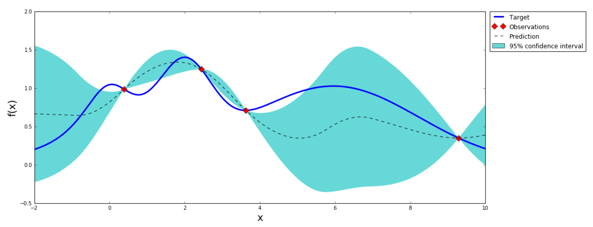
For extra fun, let's explore this time the hyper-parameter space using a Baysian Optimization (BO). BO is a constrained global optimization package built upon bayesian inference and Gaussian Processes, that attempts to find the maximum value of an unknown function in as few iterations as possible. This technique is particularly suited for optimization of high cost functions, such as training a neural network, situations where the balance between exploration and exploitation is important (see figure below). I will use the stable BayesianOptimization Python framework to implement the algorithm.
from bayes_opt import BayesianOptimization
bo = BayesianOptimization(fun, {'window': [1, 10], 'units': [1, 20]})
bo.maximize(init_points=2, n_iter=10, acq='ucb', kappa=5)
That was nice, but a bit slow, since BayesianOptimization package accepts floats as inputs, while the number of units and window size is a discrete variable. Luckily, there is another package, called hyperopt which is especially designed for hyper-parameter optimization and allows efficient exploration of discrete variable spaces.
a] LFSR-4
def fun(space):
    lfsr_4_seq = lfsr_4.run_seq(length=10000)
    x_train, x_valid, y_train, y_valid = generate_dataset(lfsr_4_seq, window=space['window'], net='recurrent')
    _, acc = train_LSTM(x_train, y_train, x_valid, y_valid, units=space['units'])
    print(space, acc)
    return acc
from hyperopt import hp, fmin, tpe
space = {'window': hp.choice('window', range(2,11)), 'units':hp.choice('units', range(1,10))}
best = fmin(fun, space, algo=tpe.suggest, max_evals=10)
b] LFSR-23
def fun(space):
    lfsr_85_seq = lfsr_85.run_seq(length=10000)
    x_train, x_valid, y_train, y_valid = generate_dataset(lfsr_23_seq, window=space['window'], net='recurrent')
    _, acc = train_LSTM(x_train, y_train, x_valid, y_valid, units=space['units'])
    print(space, acc)
    return acc
space = {'window': hp.choice('window', range(11,30,3)), 'units':hp.choice('units', range(10, 50, 5))}
best = fmin(fun, space, algo=tpe.suggest, max_evals=10)
c] LFSR-85
def fun(space):
    lfsr_85_seq = lfsr_85.run_seq(length=10000)
    x_train, x_valid, y_train, y_valid = generate_dataset(lfsr_85_seq, window=space['window'], net='recurrent')
    _, acc = train_LSTM(x_train, y_train, x_valid, y_valid, units=space['units'])
    print(space, acc)
    return acc
space = {'window': hp.choice('window', range(40,90,5)), 'units':hp.choice('units', range(10, 100, 10))}
best = fmin(fun, space, algo=tpe.suggest, max_evals=10)
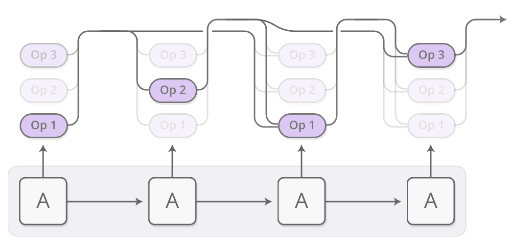
Neural Programmer
Discussion and next steps
Neural Networks learn encryption https://www.newscientist.com/article/2110522-googles-neural-networks-invent-their-own-encryption/
Compressed sensing on the program space, by enforcing sparsity (L1 norm regularization) on the weights of the operators
Test randomness of more PRGs by using Neural Programmers