Chapter 3 - Ordinary Differential Equations

(3.1) Consider the motion of a damped, driven harmonic oscillator (such as a mass on a spring, a ball in a well, or a pendulum making small motions): $m\ddot{x}+\gamma\dot{x}+kx=e^{i\omega t}.$

(a) Under what conditions will the governing equations for small displacements of a particle around an arbitrary 1D potential minimum be simple undamped harmonic motion?

From Newton's second law: $F=m\ddot{x}$.

For an 1D potential $V(x)$ we can calculate the force acting on a particle as $F=-\frac{dV(x)}{dx}$.

Assuming small perturbations ($x\rightarrow 0$), we can expand the potential as a Taylor series and keep the terms up to second order. Expanding around the minimum at $x^*$, $$V(x) = V(x)\big|_{x=x^*} + \frac{dV}{dx}x\Big|_{x=x^*} + \frac{1}{2}\frac{d^2V}{dx^2}x^2\Big|_{x=x^*} + O(x^3) = V(x)\big|_{x=x^*} + \frac{1}{2}\frac{d^2V}{dx^2}x^2\Big|_{x=x^*}$$, as $\frac{dV}{dx}x\Big|_{x=x^*} = 0$ since $x^*$ is a minimum point.

Combining the above, we have $$ m\ddot{x} = -\frac{d^2V}{dx^2}x\Big|_{x=x^*} \Rightarrow m\ddot{x} + kx = 0 $$ , with $k = -\frac{d^2V}{dx^2}\Big|_{x=x^*}$.

Which is the equation for a simple, undamped harmonic oscillator under the condition that $k\neq0$, i.e. the second derivative at the minimum should be non-zero.

(b) Find the solution to the homogeneous equation, and comment on the possible cases. How does the amplitude depend on the frequency?

Deviding by the mass, we have $$\ddot{x} + \alpha\dot{x} + \omega^2 = 0$$, where $\alpha=\frac{\gamma}{m}$ and $\omega=\sqrt{\frac{k}{m}}$.

Assuming the solution has the form $e^{\lambda t}$, and substituting above we get $$\lambda^2 + \alpha\lambda + \omega^2 = 0$$, which has the solution $$\lambda = \frac{-\alpha \pm \sqrt{\alpha^2-4\omega^2}}{2}$$

Depending on whether $\alpha^2 >,<,= 4\omega^2$ we have the well-known three cases of the harmonic oscillator (overdamped, underdamped, critically damped). A nice treatment can be found here: http://www.entropy.energy/scholar/node/damped-harmonic-oscillator

In all cases, the amplitude does not depend on the frequency.

(c) Find a particular solution to the inhomogeneous problem by assuming a response at the driving frequency, and plot its magnitude and phase as a function of the driving frequency for $m = k = 1, γ = 0.1$.

For an input $x=Ae^{i\omega t}$ we have $$-m\omega^2A+i\gamma\omega A + kA = 1$$ or $$A = \frac{1}{-m\omega^2 + i\gamma\omega + k}$$ where $$|A| = \frac{1}{\sqrt{(k-m\omega^2)^2 + \gamma^2\omega^2}}\text{ and } \phi_A = \tan^{-1}{\frac{\gamma\omega}{k-m\omega^2}}$$

Plotting for $m=k=1, \gamma=0.1$ below.

import numpy as np
import matplotlib.pyplot as plt
%matplotlib inline
m=1
k=1
gamma=.1

w= np.logspace(-1,1, num=1000)
A = 1/(-m*w**2 + 1j*gamma*w + k)
mag = 1.0/(np.sqrt((k-m*w**2)**2 + gamma**2*w**2))
# or
# mag = np.absolute(A)
phase = np.arctan2(-gamma*w,(k-m*w**2))
# or
# phase = np.angle(A)

plt.figure()
plt.semilogx (w, mag, color="blue")
plt.xlabel ("Frequency")
plt.ylabel ("Amplitude")

plt.figure()
plt.semilogx (w, phase, color="blue")
plt.xlabel ("Frequency")
plt.ylabel ("Phase")

plt.show()

(d) For a driven oscillator the $Q$ or Quality factor is defined as the ratio of the center frequency to the width of the curve of the average energy (kinetic + potential) in the oscillator versus the driving frequency (the width is defined by the places where the curve falls to half its maximum value). For an undriven oscillator the Q is defined to be the ratio of the energy in the oscillator to the energy lost per radian (one cycle is $2\pi$ radians). Show that these two definitions are equal, assuming that the damping is small. How long does it take the amplitude of a $100Hz$ oscillator with a $Q$ of $109$ to decay by $1/e$?

The average energy is the sum of the average kinetic ($T$) and potential ($U$) energies, $$\langle E\rangle = \langle T\rangle + \langle U\rangle = \frac{1}{2}m\langle\dot{x}^2\rangle + \frac{1}{2}k\langle x^2\rangle$$

Assuming a solution of the form $x = A*e^{i\omega t}=A(\cos{\omega t}+i\sin{\omega t})$, then we have (easily proven that the average of $cos^2$ and $sin^2$ in a period is $1/2$) $$\langle x^2\rangle=\frac{1}{2} \text{ and } \langle \dot{x}^2\rangle=\frac{1}{2}.$$

Thus, $$ \begin{align} \langle E\rangle &= \frac{1}{4}(m\omega^2 + k)A^2 \\ &= \frac{1}{4}\frac{m\omega^2 + k}{(k-m\omega^2) + \gamma^2\omega^2} \end{align} $$

At the center (resonant frequency) $\omega_0 = \frac{k}{m} \Rightarrow k=\omega_0m$ we have $$\langle E\rangle = \frac{1}{4m}\frac{\omega_0^2 + \omega^2}{(\omega_0^2 - \omega^2)^2 + \omega^2\gamma^2/m^2}$$

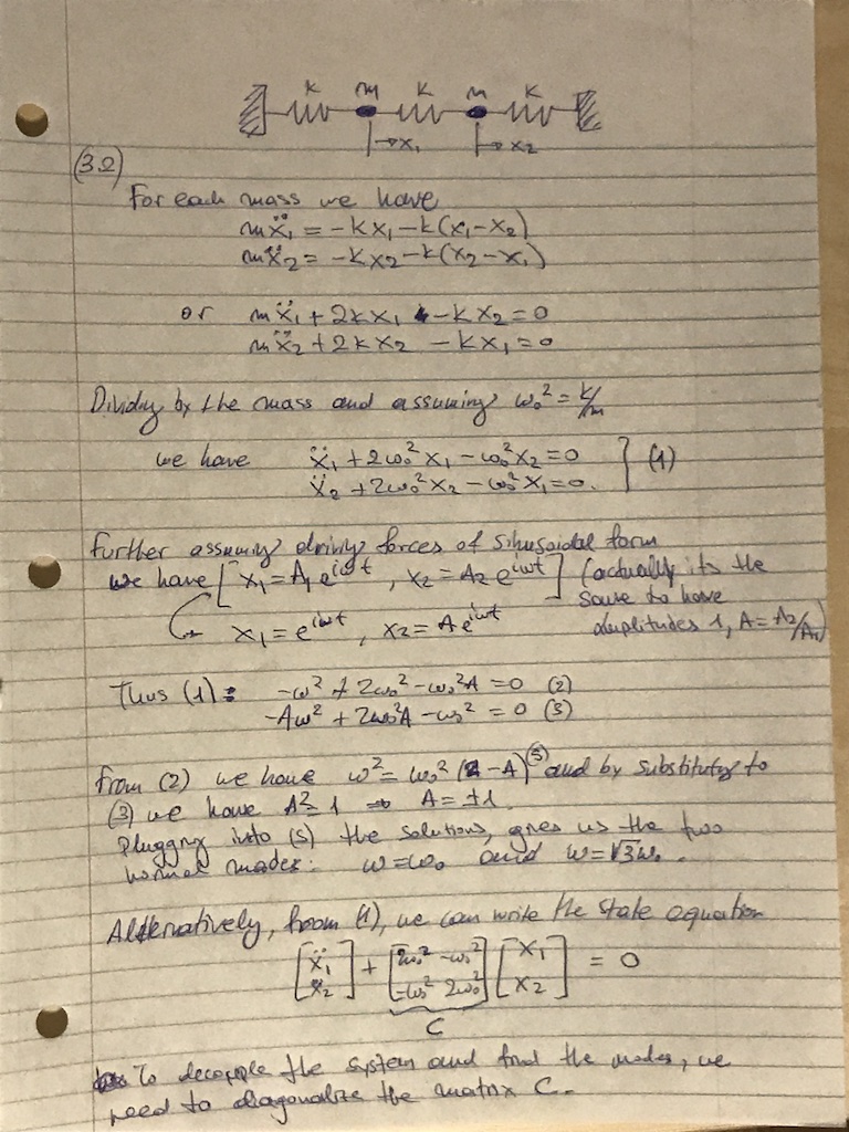
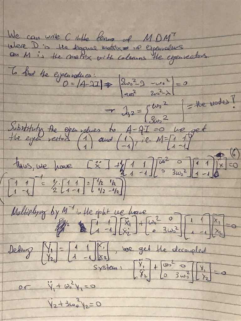
(3.2) Explicitly solve (and try to simplify) the system of differential equations for two coupled harmonic oscillators (don’t worry about the initial transient), and then find the normal modes by matrix diagonalization.

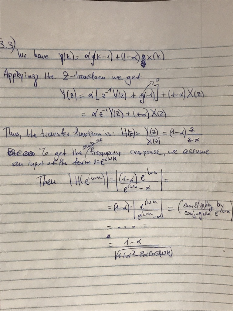
(3.3) A common simple digital filter used for smoothing a signal is $y(k)=\alpha y(k-1)+(1-\alpha)x(k)$, where $\alpha$ is a parameter that determines the response of the filter. Use $z$-transforms to solve for $y(k)$ as a function of $x(k)$ (assume $y(k<0)=0$). What is the amplitute of the frequency response?

import numpy as np
import matplotlib.pyplot as plt
%matplotlib inline

a=.01
n=1

w = np.logspace(-1,4, num=1000)
H = (1-a)*np.exp(1j*w*n)/(np.exp(1j*w*n)-a)
mag = np.absolute(H)

plt.figure()
plt.semilogx (w, mag, color="blue")
plt.xlabel ("Frequency")
plt.ylabel ("Amplitude")
plt.show()