Folding Precisely. Calculating Every Possible State of a Curved Creased Origami Tessellation.

This final project aims to deeply understand, reproduce and try to extend the current state origami curved crease tessellations from a structural point of view.

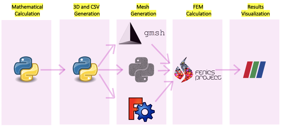
The goal of this project is to calculate mathematically the folding to be able to use it with design and simulation proposes. Te workflow proposed by this project is the following:

0. Introduction.

First of all, lets dive in a bit of a theoretical and engineering look at Origami tessellations. Inside engineering, there are tessellations everywhere. Tessellations in 2d and in 3d.

They main interest on this type of discrete structures is their capacity to fill volumes with lower density, their good structural behavior and their potential to be escalated in a easier way than a pure monolithic structure.

If we think about an origami tessellation in engineering terms, they collect all those properties and also add many others. All of them have a flat state, that means a huge potential to simplify its manufacturing, DOF can be easily tuned to generate desired motions, their capacity of changing the wet area, auxetic behaviors, etc..

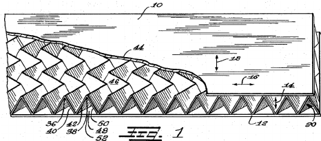
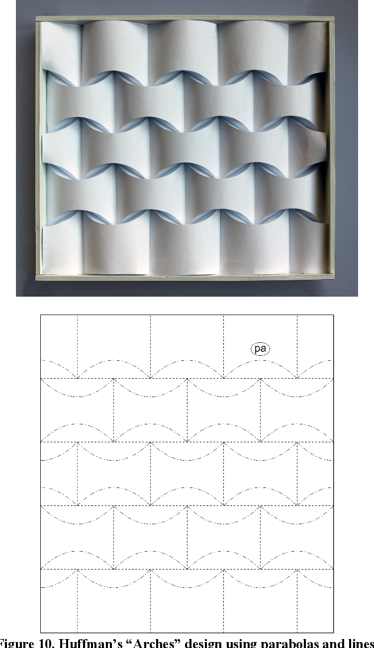
But here we are talking an specific type of Origami Tessellations. Curved creased tessellations. If the mathematics behind origami are not fully understood, curved creased foldings are even less. There are certainly active research on them as David Huffman work or Erik Demaine. The question is what is foldable and what is not foldable, and there are certainly not a unique answer for that. In the next chapter we will dive in two different answers for this question and the mathematics of an specific type of folding.

1. Mathematics.

Curved creases are a specific branch of Origami that can be explained as a Shapes of Reflection or as an infinitesimal discretization of a hinge.

The former means that any reflected shape can be foldable if when intersected by a plane, the line generated belongs to a plane at any angle of folding.

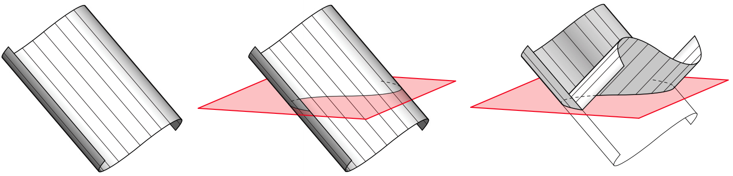
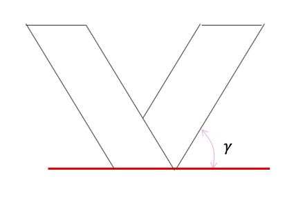
This plane, called osculating plane, generates a fold in a certain angle. The angle will be measured between the osculating plane and the ruling lines.

The following approach is based on the chapter Resilence of Sam Calisch Phd Thesis Folded functional foams.

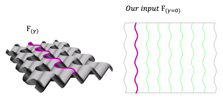
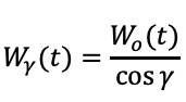
In a flat state, Fgamma is described as a semi arbitrary curve that will belong to the osculating plane when folded. We will have absolute axis and an axis evaluating the surface generated, being t the direction of the curve and W the component parallel to the ruling lines.

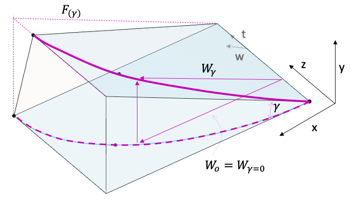
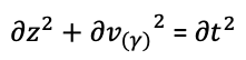
The remaining part of the triangle can be set as v(t). We also need the variation of z(t) to define the transformation of the point along the curvature. Vector t will be always normal to the ruling, the following infinitesimal relation happens:

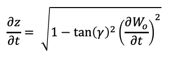
Working on the trigonometric relationship between them, the solution of the following Ordinary Differential Equation sets the z(t) values as a function of gamma and the input curve.

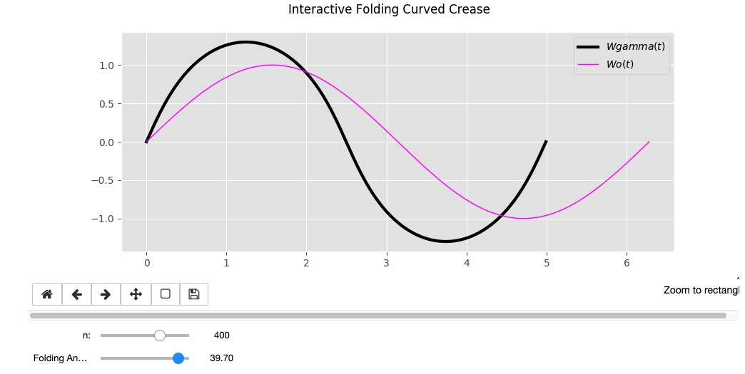
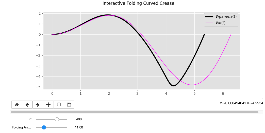
As an ODE, I have generated a script for solving the ODE using a finite difference. For this final project, Wo will be a family of sinusoidal curves. Download here to the Jupyter Notebook

The algorithm works as follows:

from sympy import *

#//////////////   Lets define here the expression of Wo we want to calculate the fold state.  /////////////

t = Symbol('t') #Defining the symbol t

Wo = sin(t) #Plug here your expression. Lets derivate it with sympy in case its get complex. 
    # IMPORTANT. Plug it in sympy notation so there is no chance to mistake. Later on we will re write it in np. 
    
dWo = diff(Wo) #Now, let derive the expression and print the result so we can manually :( translate into np. 
print(dWo)

#Importing all stuff

from sympy import *

#//////////////   Lets define here the expression of Wo we want to calculate the fold state.  /////////////
t = Symbol('t') #Defining the symbol t
Wo = sin(t) #Plug here your expression. Lets derivate it with sympy in case its get complex. 
    # IMPORTANT. Plug it in sympy notation so there is no chance to mistake. Later on we will re write it in np. 
dWo = diff(Wo) #Now, let derive the expression and print the result so we can manually :( translate into np. 
print(dWo)


import ipywidgets as widgets
from IPython.display import display
import matplotlib.pyplot as plt
from matplotlib import style


import numpy as np

%matplotlib nbagg
style.use('ggplot')

fig, ax = plt.subplots(1, figsize=(10, 4))
plt.ylim(-1.8,1.8)
plt.suptitle('Interactive Folding Curved Crease')


def Wo(t):
    return np.sin(t)
def dWodt(t):
    return np.cos(t)

def dzdt(t, y, Gamma):
    '''
    Here the function dz/dt is written. We are asking later in the euler integration the slope of the
    z(t) function at different x values.
    
    '''
    fold_ang = Gamma/180 * np.pi # Degrees
    return np.sqrt(1-(np.tan(fold_ang)**2)*((dWodt(t))**2))

def euler(n, Gamma):
    ax.clear()
    fold_ang = Gamma/180 * np.pi # Degrees
    x0 = 0 #Initial Conditions. Mandatory to solve the ODE
    y0 = 0 #Initial Conditions. Mandatory to solve the ODE
    xf = 2*np.pi #Limit of the calculation. Any value furder than 2pi will be a repetition. 
    h = (xf-x0)/n #Tiny steps definition
    x = [x0] #Array of the discrete estimated x values
    y = [y0] #Array of the discrete estimated y values

    for i in range(n):
        y0 = y0 + h * dzdt(x0,y0, Gamma)
        x0 = x0 + h
        x.append(x0)
        y.append(y0)
        
    z = []
    for i in x:
        z.append(Wo(i)/np.cos(fold_ang))
        
    ax.plot(y,z, color = 'black',linewidth = 3, label = '$Wgamma(t)$')
    ax.plot(x, Wo(x), color = 'magenta', linewidth = 1 ,label = '$Wo(t)$')
    plt.legend()
    plt.show()
    return x, y, z



n = widgets.IntSlider(min=1, max=600, value=400, description='n:')
Gamma = widgets.FloatSlider(min=0, max=45, value=0, description='Folding Angle:')
    
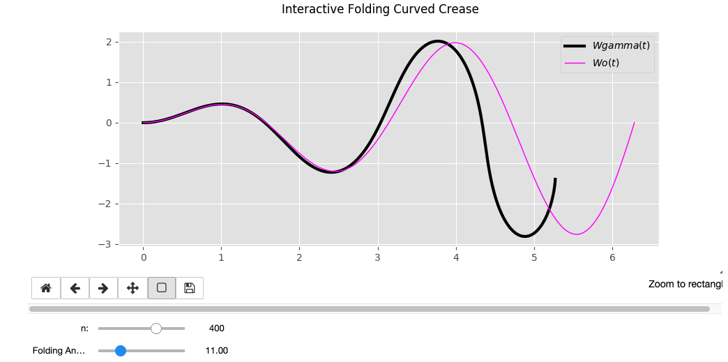
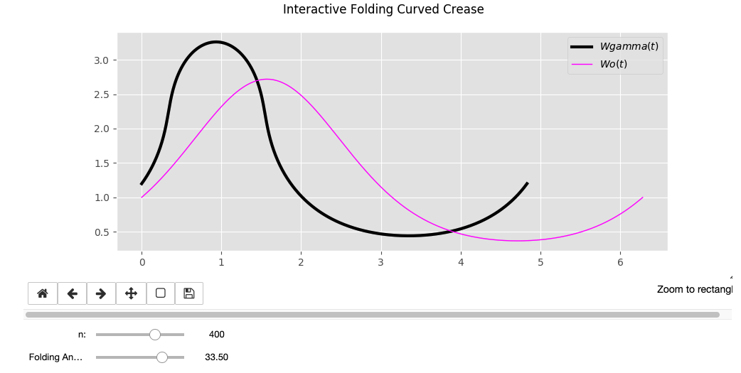
widgets.interactive(euler, n=n, Gamma=Gamma

Here you can see the output for different family of sinusoidal functions that could be folded. The

Wo = sin(t)

Wo = sin(t) * t

Wo = cos(t) * sin(t) * t

Wo = e^sin(t)

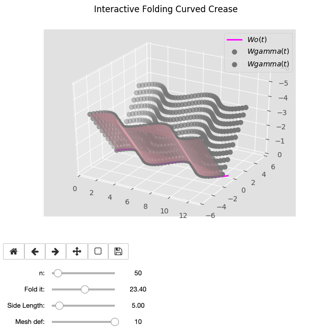
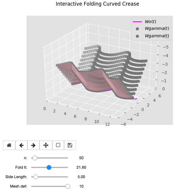
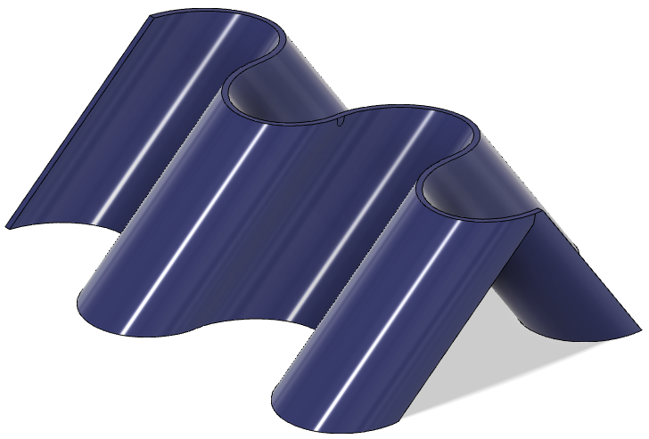
2. 3D generation and CSV export to generate STEP.

Once we have our discretized folded curves in n points, as the folding angle is just one of the primitive parameters we have been used, we can decide a goal height and loop through all the points calculated to. Download here the Jupyter notebook.

import ipywidgets as widgets
from IPython.display import display
import matplotlib.pyplot as plt
from matplotlib import style
from mpl_toolkits.mplot3d import Axes3D # <--- This is important for 3d plotting 
import numpy as np

%matplotlib nbagg
style.use('ggplot')
fig = plt.figure()
ax = fig.add_subplot( projection='3d')
plt.suptitle('Interactive Folding Curved Crease')

'''

def Wo(x):
    return np.cos(x)*np.sin(x)*x
def dWodt(x):
    return x*np.cos(2*x) + np.sin(x)*np.cos(x)

'''
def Wo(t): 
     return np.sin(t)
def dWodt(t):
    return np.cos(t)
def dzdt(t, y, Gamma):
    '''
    Here the function dz/dt is written. We are asking later in the euler integration the slope of the
    z(t) function at different x values.
    
    '''
    fold_ang = Gamma/180 * np.pi # Degrees
    return np.sqrt(1-(np.tan(fold_ang)**2)*((dWodt(t))**2))

def euler(n, Gamma, length, steps):
    ax.clear()
    fold_ang = Gamma/180 * np.pi # Degrees
    x0 = 0 #Initial Conditions. Mandatory to solve the ODE
    y0 = 0 #Initial Conditions. Mandatory to solve the ODE
    xf = 4*np.pi #Limit of the calculation. Any value furder than 2pi will be a repetition. 
    h = (xf-x0)/n #Tiny steps definition
    x = [x0] #Array of the discrete estimated x values
    y = [y0] #Array of the discrete estimated y values

    for i in range(n):
        y0 = y0 + h * dzdt(x0,y0, Gamma)
        x0 = x0 + h
        x.append(x0)
        y.append(y0)
        
    z = []
    for i in x:
        z.append(Wo(i)/np.cos(fold_ang))
    
    h = []
    for i in y:
        h.append(0)
    print(len(h))
    print(len(z))
    print(range(n+1))
    
    yp=[]
    zp=[]
    hp=[]
    
    mesh_h = length / steps
    for stp in range(steps):
        for i in range(n+1):
            y.append(y[i])
            yp.append(y[i])
            
            z.append(z[i]-stp*mesh_h*np.cos(fold_ang))
            zp.append(z[i]+stp*mesh_h*np.cos(fold_ang))

            h.append((-stp)*np.sin(fold_ang))
            hp.append((-stp)*np.sin(fold_ang))

    #Ahora tengo todos los vectores con los mismos valores. 
    
    #y,z,h = np.meshgrid(y, z,h)
    
    ax.scatter(yp,zp,hp ,color = 'grey',linewidth = 1,s=40, label = '$Wgamma(t)$')

    ax.scatter(y,z,h ,color = 'grey',linewidth = 1,s=40, label = '$Wgamma(t)$')
    ax.plot(x, Wo(x), color = 'magenta', linewidth = 2 ,label = '$Wo(t)$')
    ax.plot_trisurf(y, z, h, vmax =0.1, shade = True, color = 'pink', alpha = 0.5)
    ax.set_xlim(0,13)
    ax.set_ylim(-6,6) 
    ax.set_zlim(0,-6) 

    
    
    plt.legend()
    plt.show()
    return x, y, z



length= widgets.FloatSlider(min=0, max=45, value=5, description='Side Length:')
steps = widgets.IntSlider(min=1, max=10, value=333, description='Mesh def:')
n = widgets.IntSlider(min=1, max=600, value=50, description='n:')
Gamma = widgets.FloatSlider(min=0, max=45, value=0, description='Fold it:')
    
widgets.interactive(euler, n=n, Gamma=Gamma, length = length, steps = steps)

Wo = sin(t)

Wo = e^sin(t)

3. Meshing the generated STEP bodies

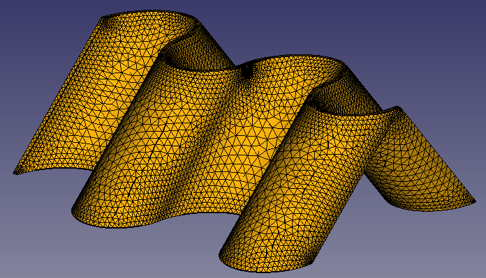
Well, meshing, and all the next points, have been a huge rabbit hole the last days. FEniCS is an awesome project but the first contact is a little bit rush. As any open source FEM sw, the requisites of the input mesh are not trivial. Also, is a program without a GUI, so you can't see physically what is being the error of the mesh while imported. Also, FEniCS is based in the solver Dolfin, that no longer gives support to transform .msh file into .xml with physical regions (loads, boundary conditions zones and any other interesting domaine to refine the mesh) information embedded. So, after many hours dealing with meshing files, gmsh, pymsh and freecad mesh, here are some thoughts that would made my life way easier if I knew them 5 days ago. My concussions are not the optimal and not the most elegant, but they work so far now.

1. The format files that FEniCS can read as a mesh are .xml and .xmdf. And right now there are differences on those formats. Open Source tools as dolfin are not supporting anymore a translation of a .msh file with physical regions into a .xml. They are translating into .xmdf.

2. So now you have a body (STEP file) you want to mesh. But FEniCS needs the mesh, and also interesting Physical Regions! In those regions, we will set Boundary Conditions and we will apply loads. Seems like there are several options to do it in FEniCS formats. Realistic stuff you can do in an afternoon learn are: - Using FreeCad mesher (later you must make a function in FEniCS specific to your mesh to specify where the clamping is happening and where the loads are being applied). For easy stuff in which you know the XYZ components of the nodes you want to clamp that ok. If your mesh is really tricky and your load is applied in a non flat weird surface, you really don't to want this at all.

3. Forget about using dolfin to run the command dolfin-convert to transform your .msh. Dolfin dont give anymore translations into xml files with physicall properties, so you better have to learn how to convert the file into xmdf. Reading xdmf in FEniCS is not the same than reading xml

4. If your body, loads or fixation belongs to a known plane, export it in FreeCad into .xml and write custom functions to define them! is the most secure option..

4. FEM in FEniCS. Such and adventure

FEniCS is an open source project that solves PDEs. Is a python tool that uses dolfin to back calculations. It provides such a solid and flexible platform to solve finite element problems.

The price to pay is that the equations must be imputed in a variational form. But there is plenty of examples and information to do all this stuff.

Briefly, here I am testing this STEP model just loading with g force due to I had some problems defining the function to apply a load in the crease (future work!)

In most platforms, FEniCS need a docker container to be used. So after installing the package with all the info here, the code to execute is the following:

We are loading here the needed libraries.

import fenics
from dolfin import *
from fenics import *
from ufl import nabla_div

Here we are defining the material constants

# Scaled variables
L = 1; W = 0.2
mu = 1
rho = 1
delta = W/L
gamma = 0.4*delta**2
beta = 1.25
lambda_ = beta
g = gamma

Now, as we told, we are importing here the mesh in xml file, and making a custom function to define boundary conditions. As we want to clamp our base, we will use a Dirichlet BC on that survace with u = (0,0,0)

# Create mesh and define function space
mesh = Mesh('test2.xml')


V = VectorFunctionSpace(mesh, 'P', 1)

# Define boundary condition
tol = 1E-14

def clamped_boundary(y, on_boundary):
    return on_boundary and y[2] < tol

bc = DirichletBC(V, Constant((0, 0, 0)), clamped_boundary)

Now, we are defining the unitary deformations and tensions

# Define strain and stress

def epsilon(u):
    return 0.5*(nabla_grad(u) + nabla_grad(u).T)
    #return sym(nabla_grad(u))

def sigma(u):
    return lambda_*nabla_div(u)*Identity(d) + 2*mu*epsilon(u)

Here, we are defining the equations into a variational problem and solve them

# Define variational problem
u = TrialFunction(V)
d = u.geometric_dimension()  # space dimension
v = TestFunction(V)
f = Constant((0, 0, -10*rho*g))
T = Constant((0, 0, 0))
a = inner(sigma(u), epsilon(v))*dx
L = dot(f, v)*dx + dot(T, v)*ds

# Compute solution
u = Function(V)
solve(a == L, u, bc)

And here we are plotting results and save all this info to be saved in a vtk file so we can open it in paraview!

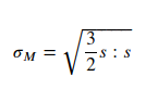
Also we are here determining von Mises tension because we do have now the displacement u solved.

# Plot solution
#plot(u, title='Displacement', mode='displacement')

# Plot stress
s = sigma(u) - (1./3)*tr(sigma(u))*Identity(d)  # deviatoric stress
von_Mises = sqrt(3./2*inner(s, s))
V = FunctionSpace(mesh, 'P', 1)
von_Mises = project(von_Mises, V)
#plot(von_Mises, title='Stress intensity')

# Compute magnitude of displacement
u_magnitude = sqrt(dot(u, u))
u_magnitude = project(u_magnitude, V)
#plot(u_magnitude, 'Displacement magnitude')
#print('min/max u:', u_magnitude.vector().array().min(), u_magnitude.vector().array().max())


V = VectorFunctionSpace(mesh, 'P', 1)

s = sigma(u) - (1./3)*tr(sigma(u))*Identity(d)
von_Mises = sqrt(3./2*inner(s, s))

#plot(von_Mises, title='Stress intensity')
vtkfile = File('results.pvd')
vtkfile << u

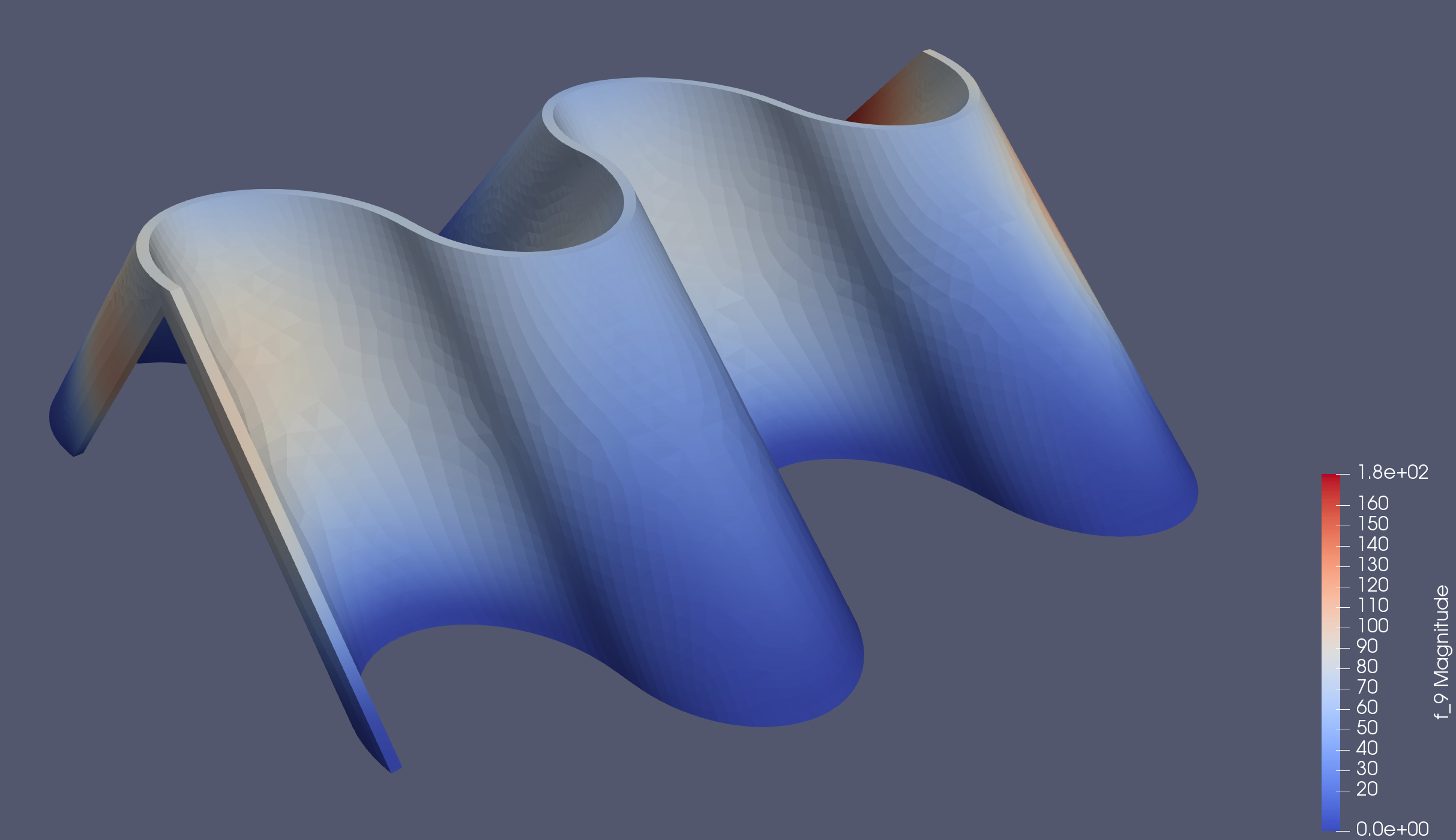
5. Paraview. Watching (enjoying) Results!

Open it in paraview, enjoy the work done!