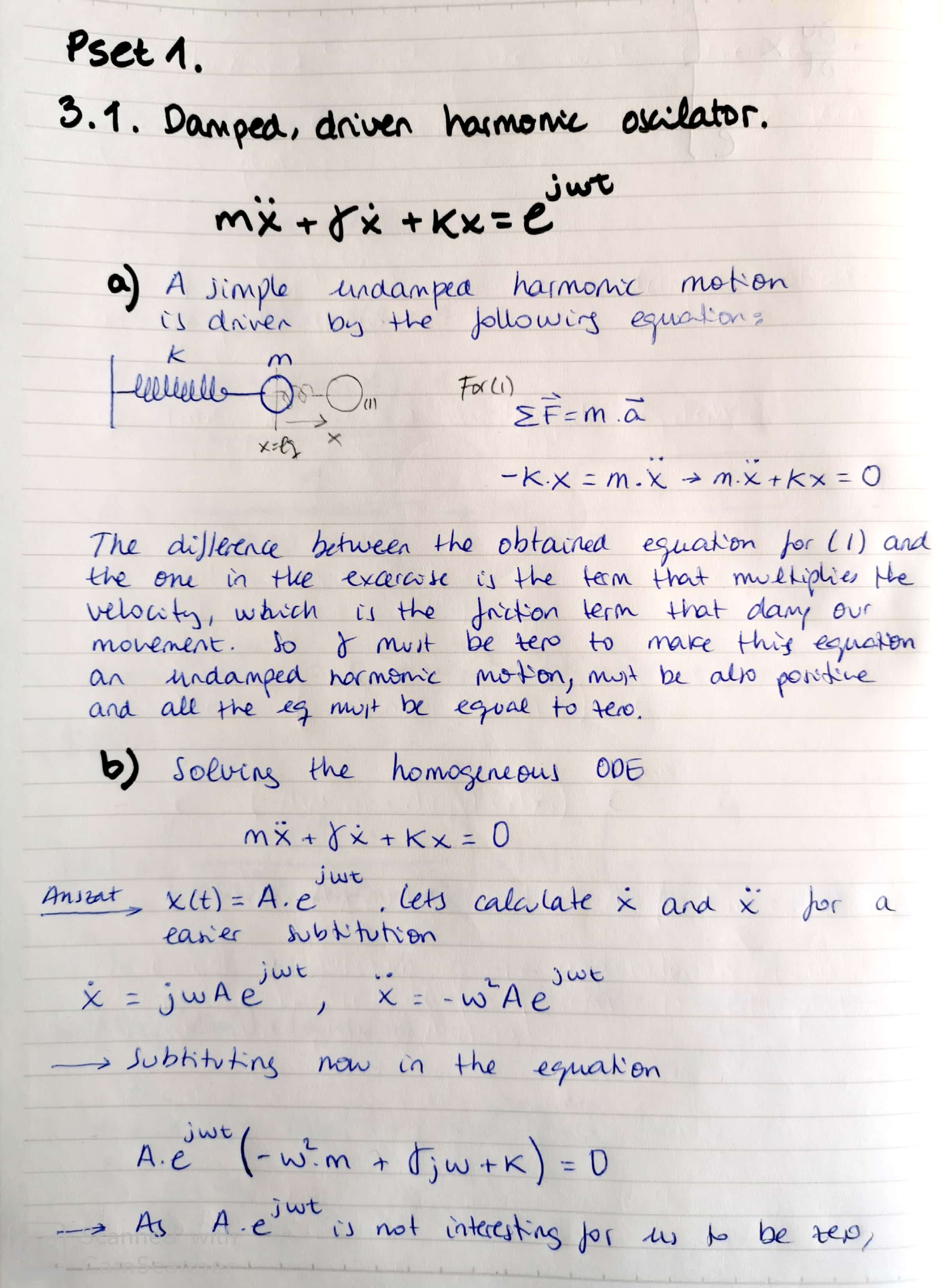
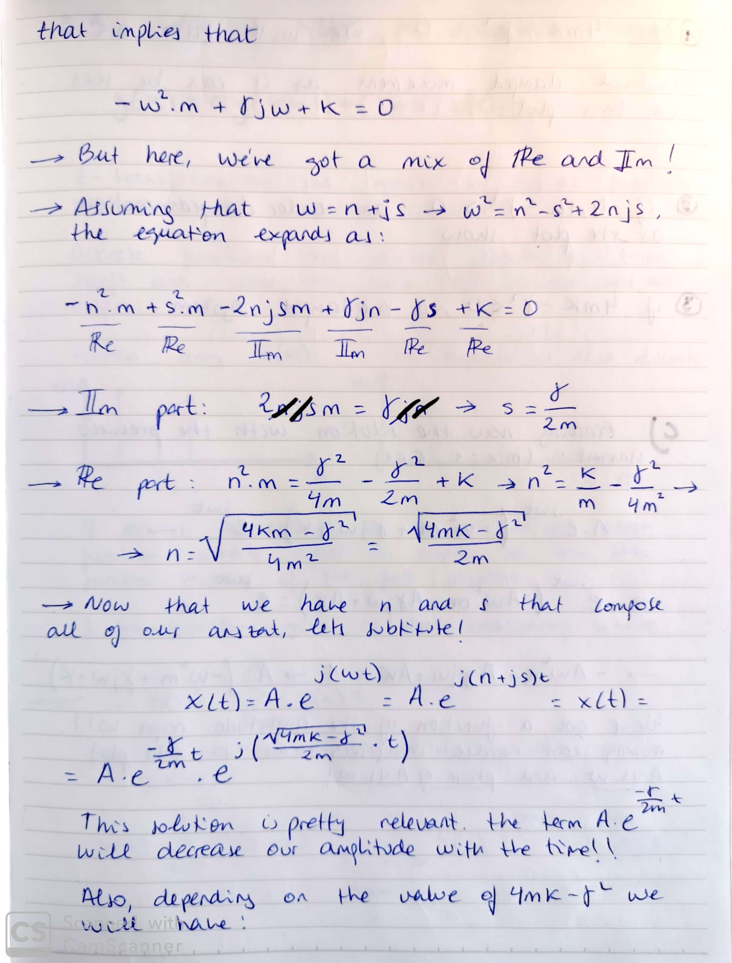
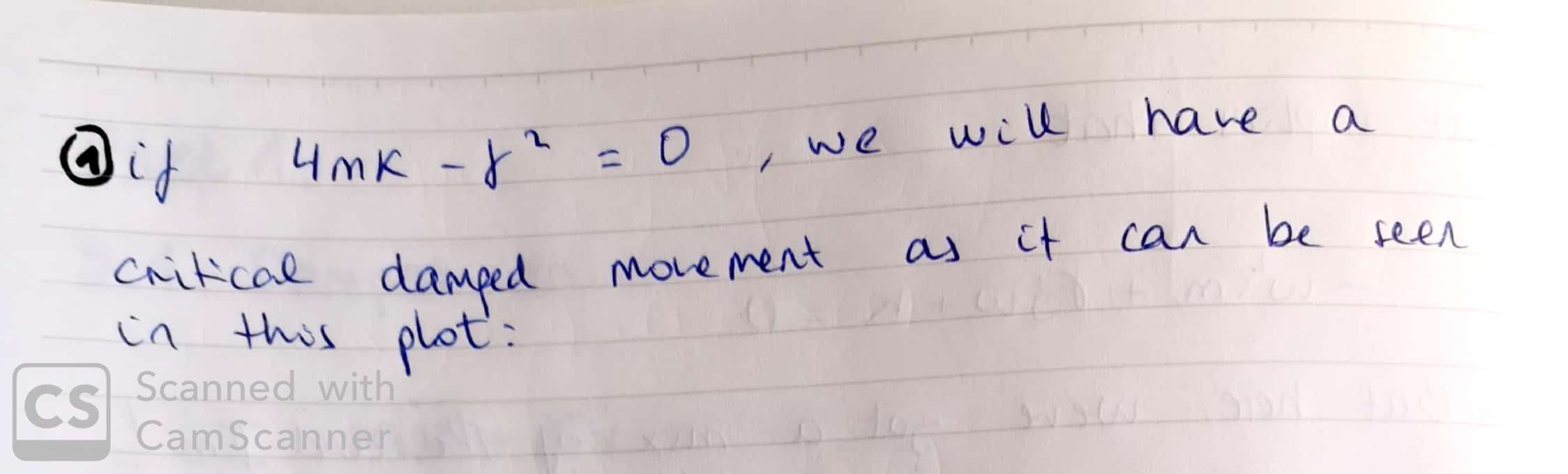
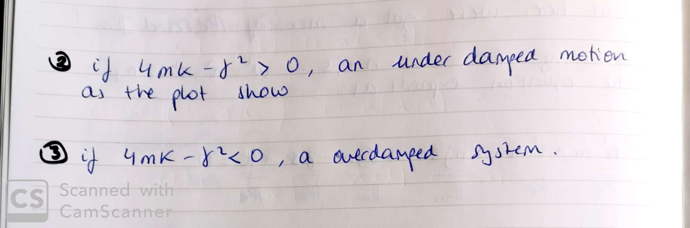
Nature of Mathematical Modelling ODEs!!!

import numpy as np
import matplotlib.pyplot as plt


x1 = np.linspace(0.0, 5.0)
x2 = np.linspace(0.0, 2.0)
A = 10


y1 = A*np.cos(2 * np.pi * x1) * np.exp(-x1)
y2 = A*np.cos(2 * 0* x1) * np.exp(-x1)

plt.subplot(2, 1, 1)
plt.plot(x1, y1, 'o-')
plt.title('A tale of 2 subplots')
plt.ylabel('Damped oscillation')

plt.subplot(2, 1, 2)
plt.plot(x2, y2, '.-')
plt.xlabel('time (s)')
plt.ylabel('Undamped')

plt.show()

import numpy as np
import matplotlib.pyplot as plt


x1 = np.linspace(0.0, 5.0)
x2 = np.linspace(0.0, 2.0)
A = 10


y1 = A*np.cos(2 * np.pi * x1) * np.exp(-x1)
y2 = A*np.cos(2 * 0* x1) * np.exp(-x1)

plt.subplot(2, 1, 1)
plt.plot(x1, y1, 'o-')
plt.title('A tale of 2 subplots')
plt.ylabel('Damped oscillation')

plt.subplot(2, 1, 2)
plt.plot(x2, y2, '.-')
plt.xlabel('time (s)')
plt.ylabel('Undamped')

plt.show()

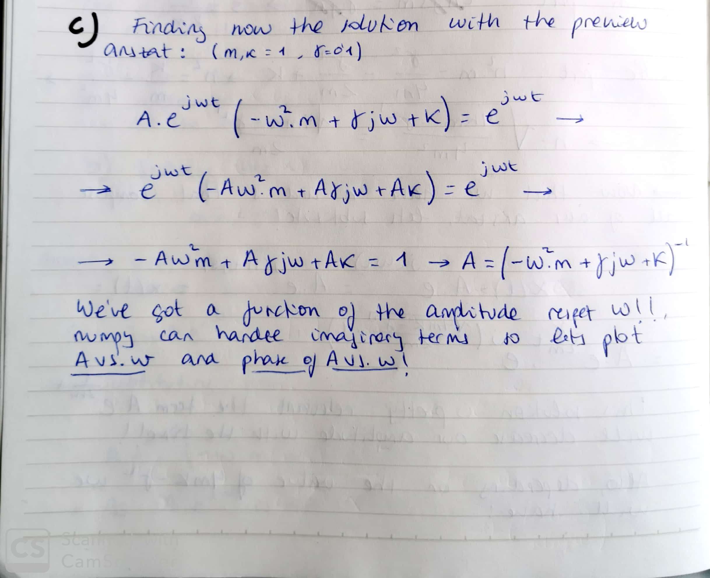
import numpy as np import matplotlib.pyplot as plt

omega = np.linspace (-5, 5, 1000)

m = 1 k = 1 gamma = 0.1

A = 1/(-momegaomega + 1jgammaomega + k)

plt.plot (omega, np.absolute(A), 'pink') plt.title('Amplitude') plt.ylabel('Damped oscillation')

plt.show()

import numpy as np
import matplotlib.pyplot as plt


omega = np.linspace (-5, 5, 1000)

m = 1
k = 1
gamma = 0.1




A = 1/(-m*omega*omega + 1j*gamma*omega + k)




plt.plot (omega, np.angle(A), 'pink')
plt.title('Amplitude')
plt.ylabel('Damped oscillation')


plt.show()

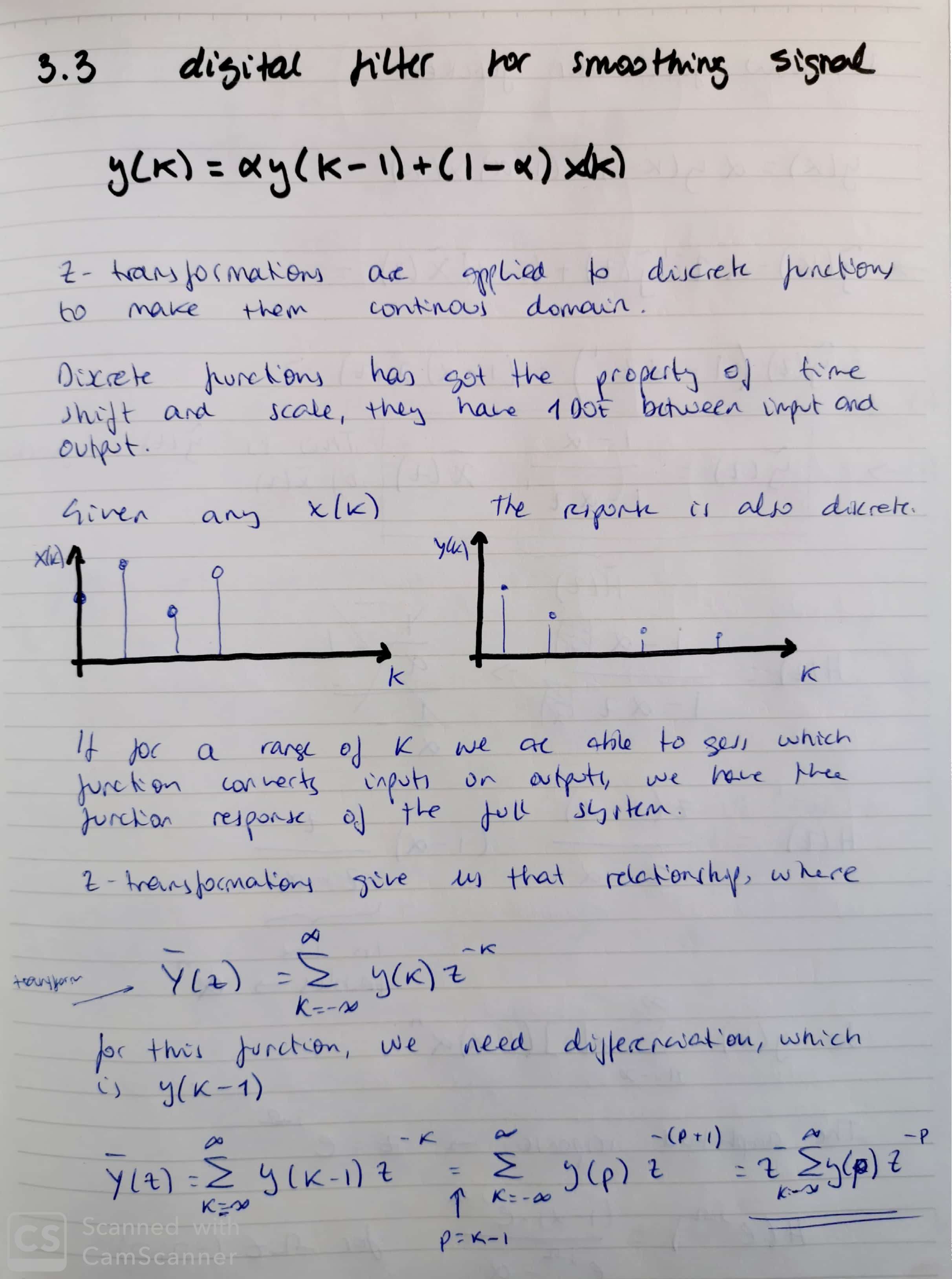
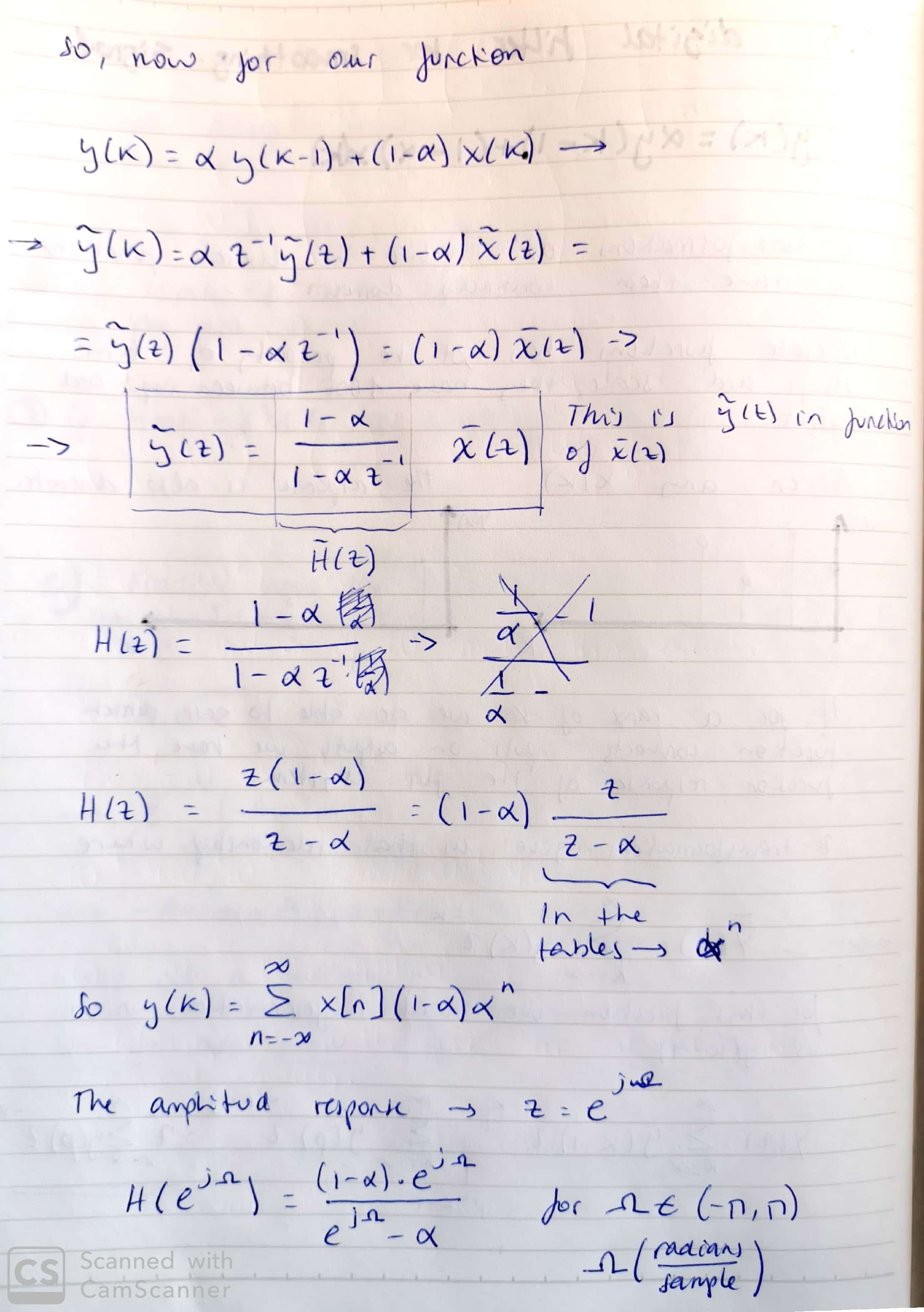
The form of the filter looks like the H function shape (amplitude responding like)

import numpy as np
import matplotlib.pyplot as plt


omega = np.linspace(-np.pi, np.pi)

alpha = 0.1

h = (1-alpha)* np.exp(1j*omega)/(np.exp(1j*omega)-alpha)


plt.plot(omega, h, 'o-')
plt.title('omega')
plt.ylabel('Damped oscillation')


plt.show()