micro - photogrammetry
motivation
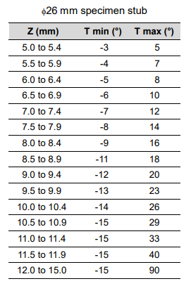
I'd like to build out a pipeline for 3D reconstruction of SEM samples. The SEM we have at CBA can be used to take mulitple images of the same sample at various tilt angles. Depending on the size of the sample and position of the stage, you can image a range of 105 degrees around the sample:
The project is motivated by a need for 3D reconstruction of filter materials in order to simulate their filtration efficiency and permeability - more details on that here.
Inspired by the algorithm described here, the piepline should follow a typical photogrammetry workflow with a few modifications for the SEM camera and simplifications due to the confined geometry of our setup.
photogrammetry background
epipolar geometry: the geometry of stereo vision - meaning mulitple 2D projections of a 3D space. The pinhole camera model is typically assumed and the optics are inverted to allow the image plane to be in between the camera and object of interest.

$O_L$ and $O_R$ are the centers of symmetry for left and right cameras respectively. $e_L$ and $e_R$ are the epipolar points (epipoles) which give the centers of symmetry for one camera in the other cameras 2D image plane, so $e_L$ is $O_R$ in the left camera. $\overline{e_RO_R}$ and $\overline{e_LO_L}$ are the epiploar lines that describe the straight forward point view that one camera sees as a line in the other camera. The plane $XO_RO_L$ that intersects all epipoles is the epipolar plane.
then we introduce homogeneous coordinates (a building block of projective geometry like cartesian coordinates for euclidean geometry) : coordinates that describe a projected plane of dimension N with N+1 points and are invariant with respect to projective transformations, i.e. any two points whose values are proportional are equivalent.
so points in the image can be described by $q = (x, y, w)$ and the transformation from homogeneous coordinates to actual (euclidean) pixel coordinates, $p$ is
$M$ is the camera intrinsics matrix and it describes the physical camera parameters
essential matrix, $E$: maps affine transformations between two camera in real space, $p \rightarrow p'$
then the fundamental matrix, $F$ relates image coordiantes from two different images to each other, bypassing the need for the intrinsic camera parameters
typical photogrammetry workflow follows these steps:
- feature extraction searches for key points that are most likely to show up across multiple pairs of images. common feature extraction methods are SIFT (Scale Invariant Feature Transform), AKAZE (Accelerated KAZE), and SURF (Speeded Up Robust Features)
- feature matching creates key points pairs accross two images. If you don't have pre-labeled calibration photos, this is typically done with a simple nearest neighboor approach and then improved upon with the RANSAC algorithm when fitting future homographies
- then, you solve for the fundamental matrix (uncalibrated images) or essential matrix (calibrated images) and the image pairs are rectified. Image rectification solves for a sepcific homography transformation that makes the epipolar lines in an image pair parallel with respect to $x$ - meaning there is no disparity in $y$. It's just a common coordinate system that simplifies the next dense mapping step to be a search in only 1 dimension as opposed to 2.
- dense mapping matches the rectified image on a pixel by pixel (or block by block for added computational efficiency) - optical flow estimations can be formed as a global energy optimization problem that outputs a disparity map between the two rectified images
- then the disparity is mapped to depth because parallax and a 3D point cloud is generated, meshed, and textured
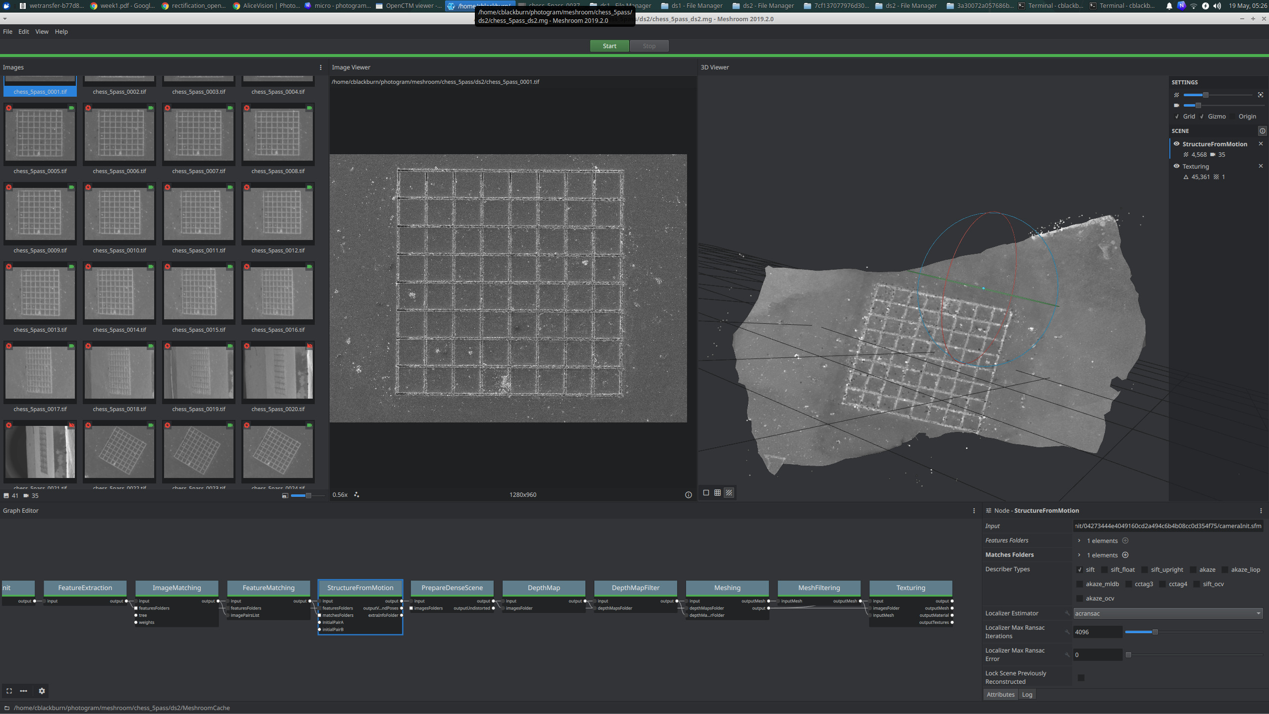
Alice Vision
Alice Vision is an open source tool for 3D reconstruction, camera tracking, and photomodeling. I thought it would be opaque and difficult to use because the documentation for Meshroom doesn't have great technical detail - but honestly it's beautiful and poking around the software is super intuitive.
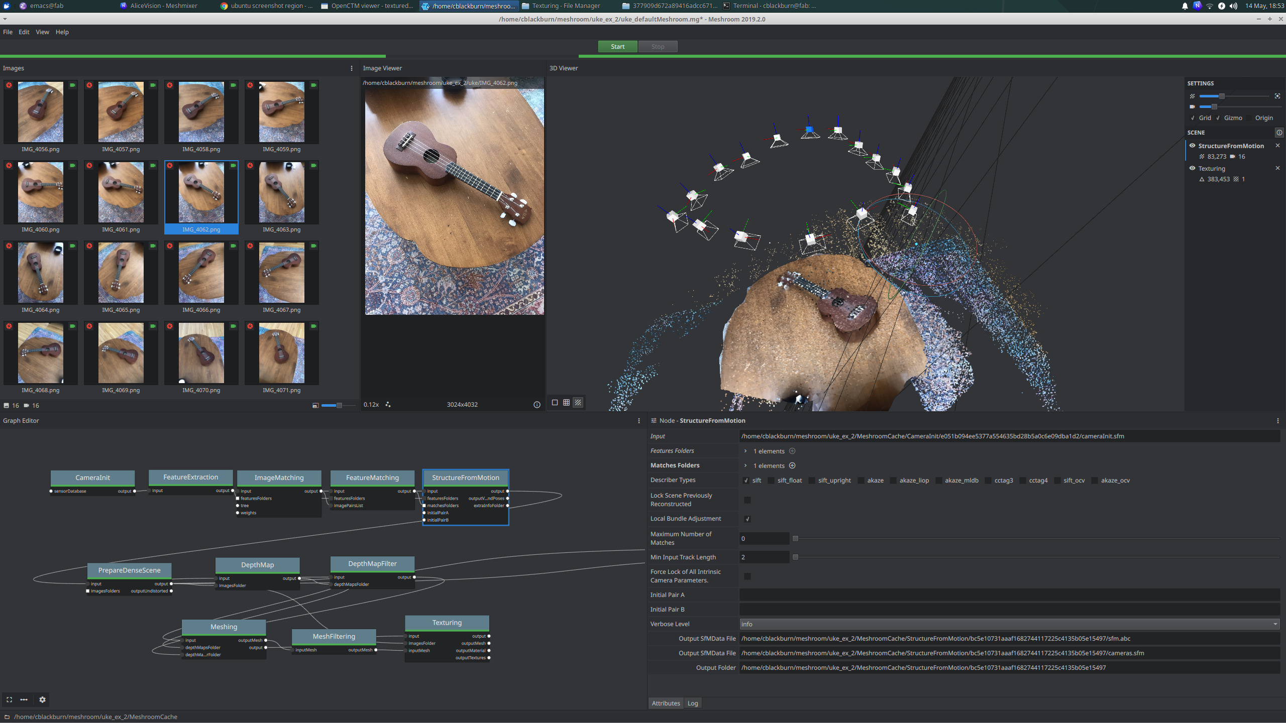
I tested it out with 16 images I quickly took with my phone of a ukelele
the model came out well and they even include nicely formatted html performance report and logs from the structure from motion step.
testing on the 300MPR filter images with minimal tilt angles (I could only get this sample to move about 6 degrees because I didn't have the chart yet matching tilt range to z-position yet).
it didn't work very well at all - even after diving into some of the advanced parameter tuning
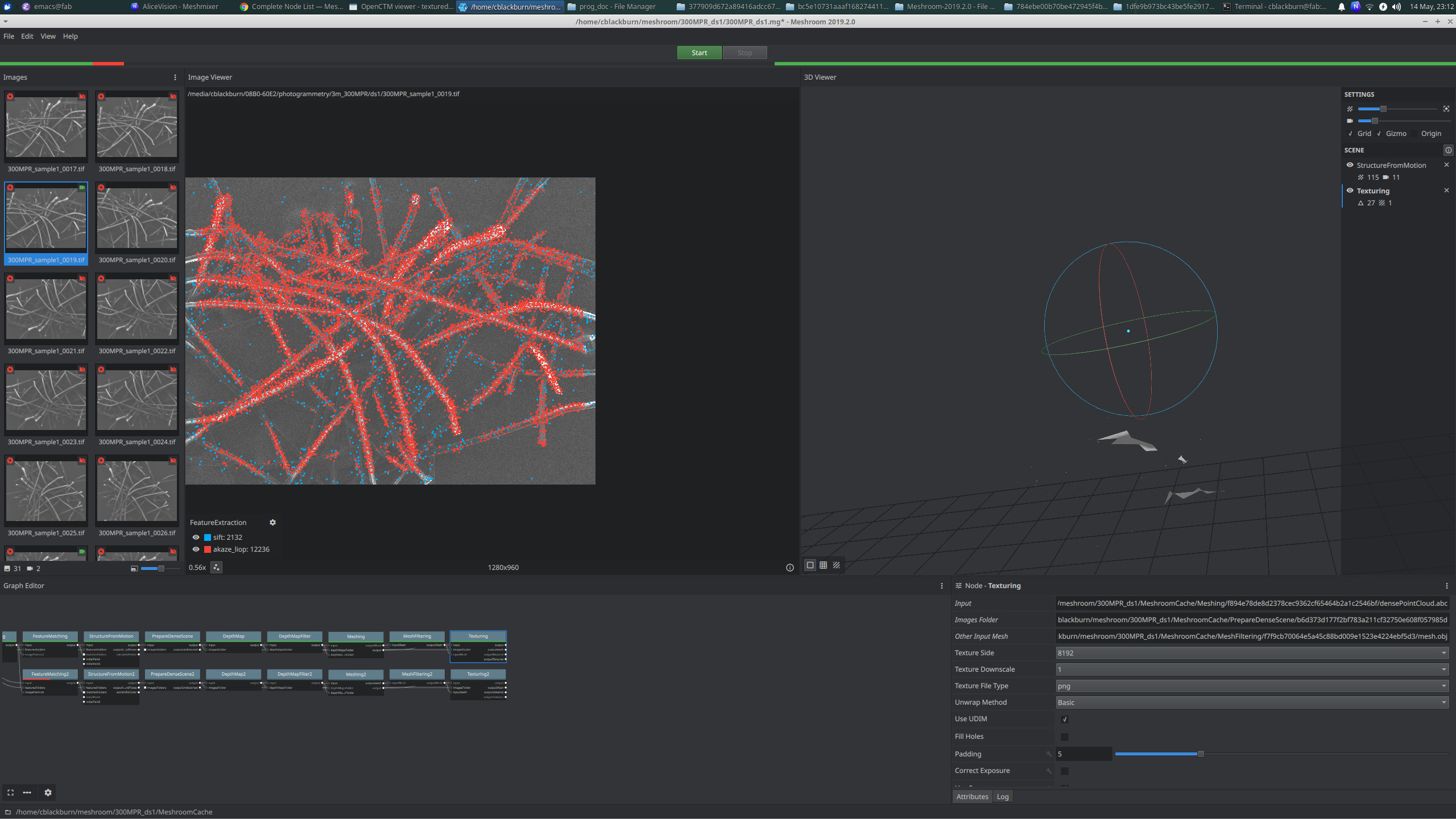
but it is interesting to see the "akaze_liop" feature estimator looks like it's picking up the individual filter fibers best . . .
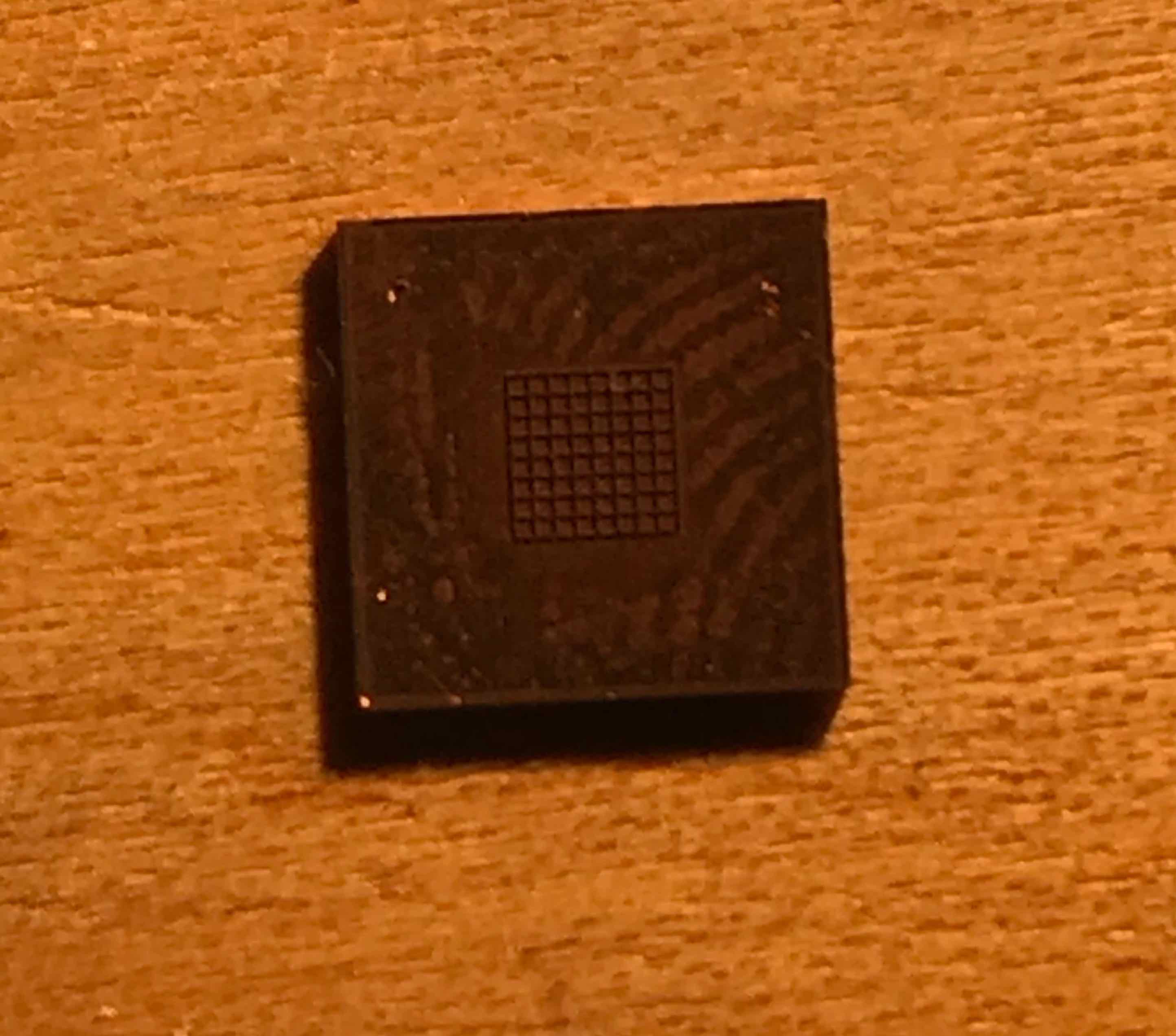
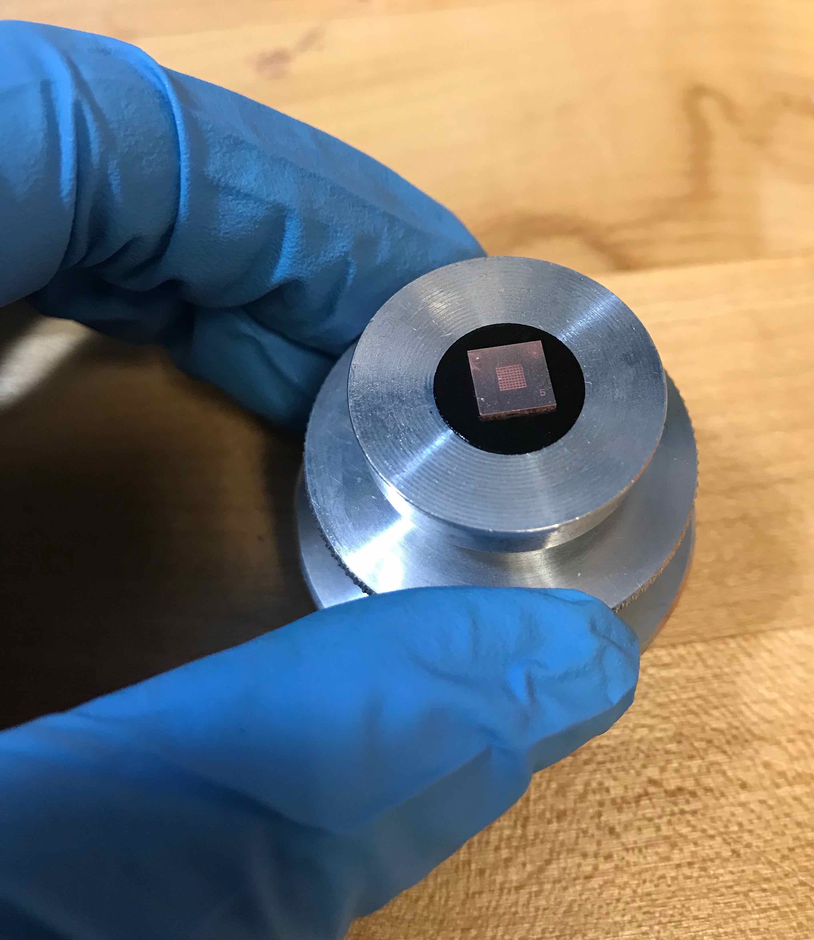
Since the fiber strands are randomly tangled and difficult to distinguish, I decided to make a small sample I could use for building the workflow and potentially calibrate the camera with.
OpenCV has a method for automatically finding the intrinsic camera matrix from a image of a chess board so i made a tiny 2mm by 2mm chess board in 0.5mm thick copper on the Oxford
With this sample, I was also able to tilt the stage much more and the Alice Vision mesh came out much nicer
openCV implementation
openCV has a ton of ready-to-go structure from motion and 3D reconstruction methods. I tried playing around with these to see if I could quickly extract the SEM intrinsic matrix from the tiny chess board I made or try to get the fundamental matrix for an image pair. The chess board didn't work :( i think the sharp edges from the laser machining throw off the edge detection in the cv2.findChessboardCorners() function. And trying to parse openCV functions felt like more of a rabbithole than just writing it out myself. i could find the fundamental matrix for two image pairs, but it looks significantly more disorted than it should be, and I'm not sure if the discrepancy is coming from the actual fundamental matrix for the cv2.warpPerspective homography transformation used to visualize it.
deeper dive into stereo rectification
Hartley and Zisserman's Multiple View geometry in Computer Vision was a great resource for this.
the fundamental matrix is defined as
where $\vec x = (x, y, 1)$ and $\vec x' = (x', y', 1)$, so expanded this has the form
which can be described by a set of homogeneous linear equations (meaning it can only be defined up to a scale)
boom we found a form to solve with SVD
but, there is an added constraint, the fundamental matrix must be singular of rank 2
recall singular vector
singular matrix is a square, non-invertible, it has a determinant of 0
just solving the linear equations will not return a singular matrix so we need to impose another constraint which is done by doing another SVD on $F$, replacing it with $F'$, and then minimizing the Frobenius norm $||F-F'||$
this is the 8-point algorithm (which was a flag in cv2.stereoREctifyUncalibrated)
- find linear solution to vec f = 0
note that this is usually not possible to solve for exactly because of noise, so you can find the result that would be closes to zero by setting $\vec f$ to be the right most singular vector corresponding to the smallest singular value of $A$, i.e. the last column of $V$.
2. impose constraint
where $D = diag(r, s, t)$ and $r \ge s \ge t$, then
adding a normalization step, this is the 8-point algorithm.
but, in order to do this we needed to at least 8 point pairs known to be matching. With a bit of added complication, you can use the RANSAC algorithm to find the fundamental matrix needing nothing except two images (i.e. no intrinsic matrix or training matches). a summary of steps are
- get some key points
- match points based on proximity and similarity in their density neighborhood
- use RANSAC as a search algorithm to generate N different $F$ using the 7-point algorithm (note we use 7-point instead of 8-point because it does not require minimzation of any norm and it's typically best practice to sue as small of a sample size as possbile with the RANSAC algorithm)
- use this F to calculate the distance, $d_\perp$ (some type of reprojectioin error) for each match
- compute inliers consiistent wtih F as coreespondences for $d_\perp \leq t$ pixels.
- then choose the F with the alrgest inliers
- use levenberg-marquardt algorithm to then re-estimate F from the correspondences that are classified as inliers, minimizing the same distance calculated in (3) for the cost evaluation.
The distance / cost function used is typically the Sampson error - it is the first order approximation of the geometric mean, which would be the ideal cost function to calculate, but it's computationally expensive and apparently the sampson does good enough.
i began implementing this, since it is the point where the openCV notebook i had was no loger making sense.
Although, i take the SIFT features as given in my code as of now, this is how they come about:
Scale Invariant Feature Transform (SIFT): feature detection algorithm consisting of four steps
- space-scale extrema detection: difference of gaussians filter at many different variances and then find local extrema to determine key points
- keypoint localization: the local extrema need to be doctored a bit to remove edges and contrast points from the key points. SEM paper does so with thresholding (also in openCV package) and quadratic function fitting. Lowe originally does so with taylor expansion?
- orientation assignment: gradient magnitude and direction is calculated for a neighborhood around the key point and a 36 bin orientation histogram is created (figure out better details in Lowe). this steps allows for better matching and confirms rotational invariance on the features
- keypoint descriptors: finally the keypoint descriptor is calculated - it's a sum of gradients weighted by a gaussian of thw 16x16 neighbors to the keypoint, split into 4x4 subregions with 8 bin histograms. so the final descriptor is 4x4x8 = 128 element vector
Implementation
work in progress . . .
define rectification class which takes a pair of images, uses the RANSAC algorithm to automatically calculate their fundamental matrix, and apply rectification homography to align x.
Find SIFT features in image pairs
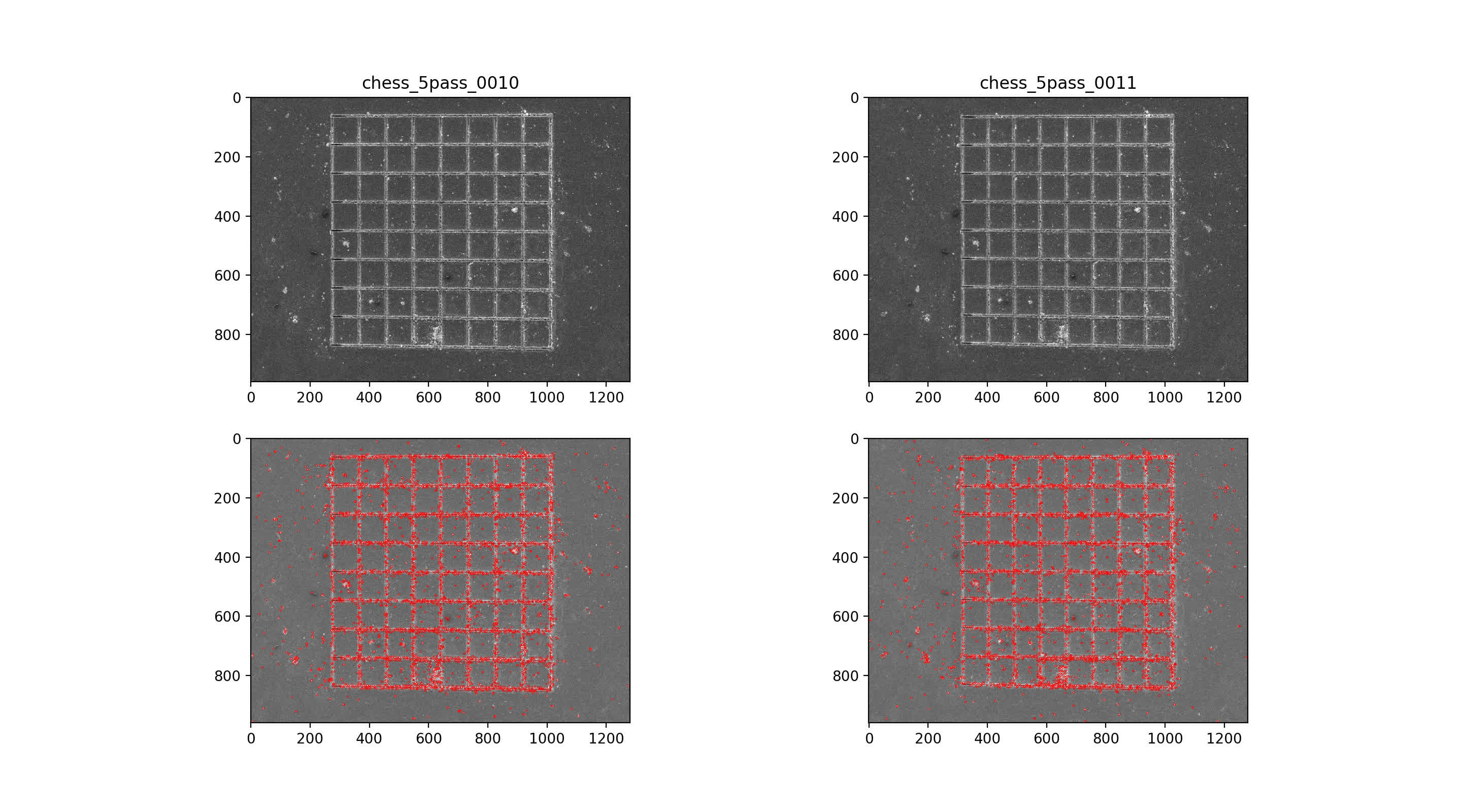

then use nearest neighbor mataching for initial putative matches, plotted across the top with max number of matches. Then, RANSAC algorithm with 7-point solution for fundamental matrix, F
9/10 img pair


10/11 img pair


rectify class::
import numpy as np
import cv2
import matplotlib.pyplot as plt
import random
import sympy as sym

class Rectify():
    def __init__(self, im1, im2):
        self.im1 = im1
        self.im2 = im2

        self.kp1, self.feat1 = self.get_features(self.im1)
        self.kp2, self.feat2 = self.get_features(self.im2)

        return

    def get_features(self, im):
        sift = cv2.xfeatures2d.SIFT_create(
            nfeatures=0,  # max features to retain
            nOctaveLayers=3, # number of layers in each octave
            contrastThreshold=0.04,  # filter out weak filters, larger --> less
            edgeThreshold=10, # filter out edge features, larger --> more
            sigma=1.6  # sigma of gaussian applied to input image at first octave
        )
        kp, feat = sift.detectAndCompute(im, None)
        return kp, feat

    def match(self, thresh=0.7):
        FLANN_INDEX_KDTREE = 0
        index_params = dict(algorithm = FLANN_INDEX_KDTREE, trees = 5)
        search_params = dict(checks = 50)
        flann = cv2.FlannBasedMatcher(index_params, search_params)

        matches = flann.knnMatch(self.feat1, self.feat2, k=2)
        good_match = []
        for m, n in matches:
            if m.distance < thresh*n.distance:
                good_match.append(m)
        return good_match

    def ransac_7pt(self, matches, inlier_thresh=1.25, plot=True):
        N = np.inf
        sample = 0
        while N > sample:
            print("sample count: ", sample)
            print("N: ", N)

            r_match = random.sample(matches, 7)
            x1 = np.float32([self.kp1[m.queryIdx].pt[0] for m in r_match])
            y1 = np.float32([self.kp1[m.queryIdx].pt[1] for m in r_match])

            x2 = np.float32([self.kp2[m.trainIdx].pt[0] for m in r_match])
            y2 = np.float32([self.kp2[m.trainIdx].pt[1] for m in r_match])

            A = np.array([x2*x1, x2*y1, x2, y2*x1, y2*y1, y2, x1, y1, np.ones(x1.shape)]).transpose()
            U, s, Vh = np.linalg.svd(A, full_matrices=True)
            V = Vh.transpose()
            #print("V: ", V)
            #print(V.shape)
            f1 = V[:, -1]
            f2 = V[:, -2]
            #print("f1: ", f1)
            #print("f2: ", f2)
            F1 = np.reshape(f1, (3, 3))
            F2 = np.reshape(f2, (3, 3))

            Fs = self.solve_F(F1, F2)

            if len(Fs) == 0:  # TO DO :: fix this
                print("no solution to fundamental matrix . . . skipping")
                continue

            print("Found fundamental matrix guesses: ", len(Fs))

            inlier_idx = []
            outlier_idx = []
            distances = []
            best_F = 0
            prev_in_count = 0
            for F in Fs:
                in_count = 0
                in_idx = []
                out_count = 0
                out_idx = []
                dist_list = []
                for i, m in enumerate(matches):
                    pt1 = self.kp1[m.queryIdx].pt
                    pt2 = self.kp2[m.trainIdx].pt
                    dist = self.sampson_dist(F, pt1, pt2)
                    dist_list.append(dist)
                    if dist < inlier_thresh:
                        in_count += 1
                        in_idx.append(i)
                    else:
                        out_count += 1
                        out_idx.append(i)
                if in_count > prev_in_count:
                    inlier_idx = in_idx
                    outlier_idx = out_idx
                    distances = dist_list
                    best_F = F
                ## TODO handle ties
                prev_in_count = in_count

            print("found ", len(inlier_idx), " inliers")
            print("found ", len(outlier_idx), " outliers")

            e = 1 - (len(inlier_idx)/len(matches))
            p = 0.99
            N = np.log(1-p)/np.log(1-(1-e)**7)
            sample += 1

        if plot:
            im_outlier, im_inlier = self.draw_ransac(matches, outlier_idx, inlier_idx)
            return best_F, im_outlier, im_inlier
        else:
            return best_F

    def sampson_dist(self, F, pt1, pt2):
        pt1 = np.array([pt1[0], pt1[1], 1])
        pt2 = np.array([pt2[0], pt2[1], 1])
        sam_num = pt2.transpose()@F@pt1
        fx1 = (F@pt1)**2
        fx2 = (F@pt2)**2
        sam = sam_num / (fx1[0] + fx1[1] + fx2[0] + fx2[1])
        return sam

    def sampson_err(self, F, pts1, pts2):
        '''
        calculate sampson error - the first order approximation to geometric error
        '''
        err = 0
        for i in range(pts1.shape[0]):
            sam_num = (pts2[i, :].transpose()@F@pts1[i, :])**2
            fx1 = F@pts1[i, :]**2
            fx2 = F.transpose()@pts2[i, :]**2
            sam = sam_num / (fx1[0] + fx1[1] + fx2[0] + fx2[1])
            err += sam
        return err


    def solve_F(self, F1, F2):
        '''
        solve for det(alpha*F1 + (1-alpha)*F2) = 0 for
        7 point fundamental matrix subject to rank 2 constraint

        returns 1 or 3 values (degeneracy but ignore complex values)
        '''
        #F1 = sym.Matrix(F1)
        #F2 = sym.Matrix(F2)
        #a = sym.symbols('a', real=True)
        a = sym.symbols('a')
        M = a*F1 + (1-a)*F2
        #print("array M", M)
        M = sym.Matrix(M)
        #print("matrix M", M)
        #print("determ ", M.det())
        alphas = sym.solve(M.det(), a)
        print("all alphas: ", alphas)
        filter_a = []
        for i, alpha in enumerate(alphas):
            if abs(sym.im(alpha)) < 1e-20:
                filter_a.append(np.float64(sym.re(alpha)))
            else:
                continue
        print("filtered alphas: ", filter_a)
        Fs = [(a*F1 + (1-a)*F2) for a in filter_a]

        return Fs


    ################
    ## plot helpers
    ###############

    def draw_matches(self, matches):
        draw_params = dict(
            matchColor = (0, 0, 255),
            singlePointColor = (0, 255, 0),
            flags = 0
        )
        im = cv2.drawMatches(self.im1, self.kp1, self.im2, self.kp2, matches, None, **draw_params)
        cv2.putText(im, "num matches: %s" % len(matches), (10, 50),
                    cv2.FONT_HERSHEY_SIMPLEX, 2, (0, 0, 0), 4
        )
        return im

    def draw_keypoints(self, side=1, color=[255, 0, 0]):
        if side == 1:
            im = np.zeros(self.im1.shape)
            im = cv2.drawKeypoints(self.im1, self.kp1, im, color=color)
        if side == 2:
            im = np.zeros(self.im2.shape)
            im = cv2.drawKeypoints(self.im2, self.kp2, im, color=color)
        return im

    def draw_ransac(self, matches, outlier_idx, inlier_idx):
        font=cv2.FONT_HERSHEY_SIMPLEX
        fontScale=2
        color=(0, 0, 0)
        thickness = 4
        im_outlier = cv2.cvtColor(self.im1, cv2.COLOR_GRAY2RGB)
        for out in outlier_idx:
            start = self.kp1[matches[out].queryIdx].pt
            start = (round(start[0]), round(start[1]))
            stop = self.kp2[matches[out].trainIdx].pt
            stop = (round(stop[0]), round(stop[1]))
            cv2.circle(im_outlier, start, 6, (0, 255, 0), thickness=-5)
            cv2.line(im_outlier, start, stop, (255, 0, 0), 4)
        cv2.putText(im_outlier, "num outliers: %s" % len(outlier_idx), (10, 50),
                    font,
                    fontScale,
                    color,
                    thickness
        )
        im_inlier = cv2.cvtColor(self.im1, cv2.COLOR_GRAY2RGB)
        for inl in inlier_idx:
            start = self.kp1[matches[inl].queryIdx].pt
            start = (round(start[0]), round(start[1]))
            stop = self.kp2[matches[inl].trainIdx].pt
            stop = (round(stop[0]), round(stop[1]))
            cv2.circle(im_inlier, start, 6, (0, 255, 0), thickness=-5)
            cv2.line(im_inlier, start, stop, (255, 0, 0), 4)
        cv2.putText(im_inlier, "num inliers: %s" % len(inlier_idx), (10, 50),
                    font,
                    fontScale,
                    color,
                    thickness
        )
        return im_outlier, im_inlier