Problem Set 2 (ODEs)

1

Consider the motion of a damped, driven harmonic oscillator (such as a mass on a spring, a ball in a well, or a pendulum making small motions):

$m \ddot{x} + \gamma \dot{x} + kx = e^{i \omega t}$

(a)

Under what conditions will the governing equations for small displacements of a particle around an arbitrary 1D potential minimum be simple undamped harmonic motion?

WLOG assume the potential minimum is at $x = 0$ . Undamped simple harmonic motion occurs when $F = -kx$ . Since the force a particle experiences due to a potential $U(x)$ is $F = -\frac{d}{dx} U(x)$ , this means we’ll get simple harmonic motion when $\frac{d}{dx} U(x) = kx$ . Thus

$U(x) = U(0) + \frac{k}{2} x^2$

So formally there are two free parameters, but the constant term is meaningless from a physics perspective because it drops out of all the governing equations. (Interestingly not all constant terms in potentials are physically irrelevant — as we learned in PIT last year, the magnetic vector potential itself is observable via the Aharanov-Bohm effect.)

Close to the local minimum at $x = 0$ , we can write an arbitrary potential as

$U(x) = U(0) + \frac{\ddot{U}(0)}{2!} x^2 + \frac{\ddot{U}(0)}{3!} x^3 + \ldots$

( $\dot{U}(0)$ has to be zero as otherwise $x = 0$ isn’t a local minimum.) So another characterization is that simple harmonic motion results when all derivatives of $U$ are zero except the second. However for any potential with no linear term and a nonvanishing quadratic term, for sufficiently small $x$ all the higher order terms are negligible, so simple harmonic motion will still be a good approximation near the minimum.

(b)

Find the solution to the homogeneous equation, and comment on the possible cases. How does the amplitude depend on the frequency?

The homogeneous version is

$m \ddot{x} + \gamma \dot{x} + kx = 0$

Using the ansatz $x(t) = e^{rt}$ , this equation becomes

$m r^2 + \gamma r + k = 0$

which is solved by

$r = \frac{-\gamma \pm \sqrt{\gamma^2 - 4mk}}{2m}$

There are three main cases.

Assuming these two roots are distinct, the general solution is

$\begin{aligned} x(t) &= Ae^{r_1 t} + Be^{r_2 t} \\ &= Ae^{\frac{-\gamma + \sqrt{\gamma^2 - 4mk}}{2m} t} + Be^{\frac{-\gamma - \sqrt{\gamma^2 - 4mk}}{2m} t} \\ &= e^{-\frac{\gamma}{2m} t} \left( A e^{\frac{\sqrt{\gamma^2 - 4mk}}{2m} t} + B e^{-\frac{\sqrt{\gamma^2 - 4mk}}{2m} t} \right) \end{aligned}$

Over-damped

If $\gamma^2 > 4mk$ , then the square root is real. So the solution is entirely exponential growth and/or decay. In the typical case where $\gamma$ and $k$ are positive, the solution quickly ends up dominated by the exponential decay up front. This is called an over-damped system.

Under-damped

If $\gamma^2 < 4mk$ , then the square root is imaginary. So the solution is oscillatory with exponential growth or decay of the amplitude. In the typical scenario it will be exponential decay. This is called an under-damped system.

Critically damped

If $\gamma^2 = 4mk$ , then the general solution above isn’t valid since we have a double root $r = -\frac{\gamma}{2m}$ . So we have to add a factor of $t$ to the ansatz to get the second term.

$\begin{aligned} x(t) &= Ae^{rt} + Bte^{rt} \\ &= (A + Bt) e^{rt} \\ &= (A + Bt) e^{-\frac{\gamma}{2m} t} \end{aligned}$

This is a single term of exponential growth or decay. In the typical situation it represents decay, and the system is critically damped.

(c)

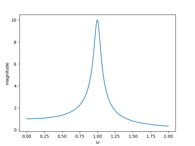
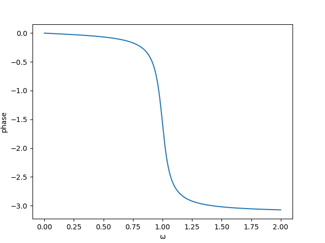
Find a particular solution to the inhomogeneous problem by assuming a response at the driving frequency, and plot its magnitude and phase as a function of the driving frequency for $m = k = 1$ , $\gamma = 0.1$ .

Now we’re solving the full ODE:

$m \ddot{x} + \gamma \dot{x} + kx = e^{i \omega t}$

Start with the ansatz $x(t) = A e^{i \omega t}$ . The equation reduces to

$-m \omega^2 A + i \gamma \omega A + k A = 1$

$A = \frac{1}{-m \omega^2 + i \gamma \omega + k}$

Thus the general solution to the inhomogeneous problem (assuming distinct roots) is

$x(t) = e^{-\frac{\gamma}{2m} t} \left( A e^{\frac{\sqrt{\gamma^2 - 4mk}}{2m} t} + B e^{-\frac{\sqrt{\gamma^2 - 4mk}}{2m} t} \right) + \frac{1}{-m \omega^2 + i \gamma \omega + k} e^{i \omega t}$

Here are plots of the magnitude and phase of the particular solution.

amplitude

phase

(d)

For a driven oscillator the Q or Quality factor is defined as the ratio of the center frequency to the width of the curve of the average energy (kinetic + potential) in the oscillator versus the driving frequency (the width is defined by the places where the curve falls to half its maximum value). For an undriven oscillator the Q is defined to be the ratio of the energy in the oscillator to the energy lost per radian (one cycle is $2\pi$ radians). Show that these two definitions are equal, assuming that the damping is small. How long does it take the amplitude of a 100 Hz oscillator with a Q of 109 to decay by $1/e$ ?

Undriven

As we found previously, the general solution is

$x(t) = e^{-\frac{\gamma}{2m} t} \left( A e^{\frac{\sqrt{\gamma^2 - 4mk}}{2m} t} + B e^{-\frac{\sqrt{\gamma^2 - 4mk}}{2m} t} \right)$

To clean things up a bit, let’s define

$\begin{aligned} \omega_0 &= \sqrt{k/m} \\ \alpha &= \frac{\gamma}{2 m} \end{aligned}$

Then

$\frac{\sqrt{\gamma^2 - 4mk}}{2m} = \sqrt{\alpha^2 - \omega_0^2}$

Since we’re assuming low damping, $\alpha^2 - \omega_0^2$ is negative. So we’ll use

$\sqrt{\alpha^2 - \omega_0^2} = i \sqrt{\omega_0^2 - \alpha^2}$

Finally, to be as lazy as possible, we’ll define $\omega_1^2 = \omega_0^2 - \alpha^2$ (which is a positive real number). All together this compresses our general solution to

$\begin{aligned} x(t) &= e^{-\alpha t} \left( A e^{\sqrt{\alpha^2 - \omega_0^2} t} + B e^{-\sqrt{\alpha^2 - \omega_0^2} t} \right) \\ &= e^{-\alpha t} \left( A e^{i \sqrt{\omega_0^2 - \alpha^2} t} + B e^{-i \sqrt{\omega_0^2 - \alpha^2} t} \right) \\ &= e^{-\alpha t} \left( A e^{i \omega_1 t} + B e^{-i \omega_1 t} \right) \\ \end{aligned}$

But this form won’t work so well for us here, since it involves complex numbers. In particular, if we only wanted to apply linear operations to the solutions, we could just take their real parts at the end of the day. But energy depends nonlinearly on the function (i.e. $m\dot{x}^2$ ), so the real and imaginary terms would interfere. So to make sure the physics makes sense, we had best stick to real solutions.

Since this is a linear homogeneous ODE, the real and imaginary parts by themselves are both solutions to the system (see my notes for why this works). So using the Euler identity $e^{ix} = \cos(x) + i \sin(x)$ , we can find a general form for the real solutions.

$x(t) = e^{-\alpha t} (A \cos(\omega_1 t) + B \sin(\omega_1 t))$

The energy in the system is the sum of the kinetic and potential energies.

$E = \frac{1}{2} m \dot{x}^2 + \frac{1}{2} k x^2$

It’s easy enough to see that

$x^2(t) = e^{-2 \alpha t} (A \cos(\omega_1 t) + B \sin(\omega_1 t))^2$

Applying the product rule to the general form as written above, and doing some tedious bookkeeping, we can also find the $\dot{x}$ terms we need for the energy of the system.

$\begin{aligned} \dot{x}(t) &= -e^{-\alpha t} \left[ \alpha (A \cos(\omega_1 t) + B \sin(\omega_1 t)) + \omega_1 (A \sin(\omega_1 t) - B \cos(\omega_1 t)) \right] \\ \dot{x}(t)^2 &= e^{-2 \alpha t} \left[ \alpha (A \cos(\omega_1 t) + B \sin(\omega_1 t)) + \omega_1 (A \sin(\omega_1 t) - B \cos(\omega_1 t)) \right]^2 \end{aligned}$

The general formula for energy is quite messy, but the initial energy isn’t so bad.

$E(0) = \frac{1}{2} m \left( A \alpha - B \omega_1 \right)^2 + \frac{1}{2} k A^2$

Notice how this still has a term that looks like $\frac{1}{2} m v^2$ , and one that looks like $\frac{1}{2} k x^2$ . The units work out too: as sufficiently paranoid physicists have already checked, $\alpha$ and $\omega$ are in inverse seconds, while $A$ is in meters.

To compute the change in the energy of the system, we’d like to integrate $dE/dt$ . Note that

$\begin{aligned} E &= \frac{1}{2} m \dot{x}^2 + \frac{1}{2} k x^2 \\ \frac{dE}{dt} &= m \dot{x} \ddot{x} + k x \dot{x} \\ &= \dot{x} (m \ddot{x} + k x) \\ &= -\gamma \dot{x}^2 \end{aligned}$

The last line follows because the ODE governing the system says $m \ddot{x} + k x = -\gamma \dot{x}$ .

So the change in energy over one cycle is

$\begin{aligned} \Delta E &= \gamma \int_0^\frac{2 \pi}{\omega_1} \dot{x}(t)^2 dt \\ &= \gamma \int_0^\frac{2 \pi}{\omega_1} e^{-2 \alpha t} [ \alpha (A \cos(\omega_1 t) + B \sin(\omega_1 t)) \\ &\hphantom{\gamma \int_0^\frac{2 \pi}{\omega_1}} + \omega_1 (A \sin(\omega_1 t) - B \cos(\omega_1 t)) ]^2 dt \\ &\approx \gamma \int_0^\frac{2 \pi}{\omega_1} [ \alpha (A \cos(\omega_1 t) + B \sin(\omega_1 t)) \\ &\hphantom{\gamma \int_0^\frac{2 \pi}{\omega_1}} + \omega_1 (A \sin(\omega_1 t) - B \cos(\omega_1 t)) ]^2 dt \end{aligned}$

I’m dropping the minus sign since I want the magnitude of the change (the absolute change is negative since the system is losing energy). And since $\gamma$ is small, over one cycle the exponential term is basically constant with a value of 1. So I dropped it. After some math, we find

$\Delta E = \frac{\pi \gamma}{\omega_1} \left(A^2 \alpha^2 + B^2 \alpha^2 + \omega_1^2 \left(A^2 + B^2\right)\right)$

So finally $Q$ is

$\begin{aligned} Q &= 2 \pi \frac{E(0)}{\Delta E} \\ &= \frac{\omega_1 \left(A^2 k + m \left(A \alpha - B \omega_1 \right)^2 \right)} {\gamma \left(A^2 \alpha^2 + B^2 \alpha^2 + \omega_1^2 \left(A^2 + B^2 \right) \right)} \\ &\approx \frac{\omega_1 \left(A^2 k + m \left(B \omega_1 \right)^2 \right)} {\gamma \omega_1^2 \left(A^2 + B^2 \right) } \\ &\approx \frac{A^2 k + m \omega_0^2 B^2}{\gamma \omega_0 \left(A^2 + B^2 \right) } \\ &= \frac{k \left( A^2 + B^2 \right)}{\gamma \omega_0 \left(A^2 + B^2 \right) } \\ &= \frac{k}{\gamma \omega_0^2} \\ &= \frac{\sqrt{km}}{\gamma} \end{aligned}$

The factor of $2 \pi$ is to normalize $\Delta E$ per radian rather than cycle. Two different approximations are used. First, $\alpha$ is basically zero. Second, $\omega_1$ is basically $\omega_0$ . And $m \omega_0^2 = k$ .

(e)

Now find the solution to equation (3.58) by using Laplace transforms. Take the initial condition as $x(0) = \dot{x}(0) = 0$ .

Using the table in the book, and keeping in mind the initial conditions, I found the following transforms.

$\begin{aligned} \mathcal{L}[m \ddot{x}(t)] &= m \left( s^2 X(s) - s x(0) - \dot{x}(0) \right) \\ &= m s^2 X(s) \\ \mathcal{L}[\gamma \dot{x}(t)] &= \gamma \left( s X(s) - x(0) \right) \\ &= \gamma s X(s) \\ \mathcal{L}[k x(t)] &= k X(s) \\ \mathcal{L}[e^{i \omega t}] &= \frac{1}{s - i \omega} \end{aligned}$

So our transformed ODE is

$m s^2 X(s) + \gamma s X(s) + k X(x) = \frac{1}{s - i \omega} \\ X(s) = \frac{1}{(s - i \omega) (m s^2 + \gamma s + k)}$

Now it’s just a bunch of algebra and an inverse transform…

(f)

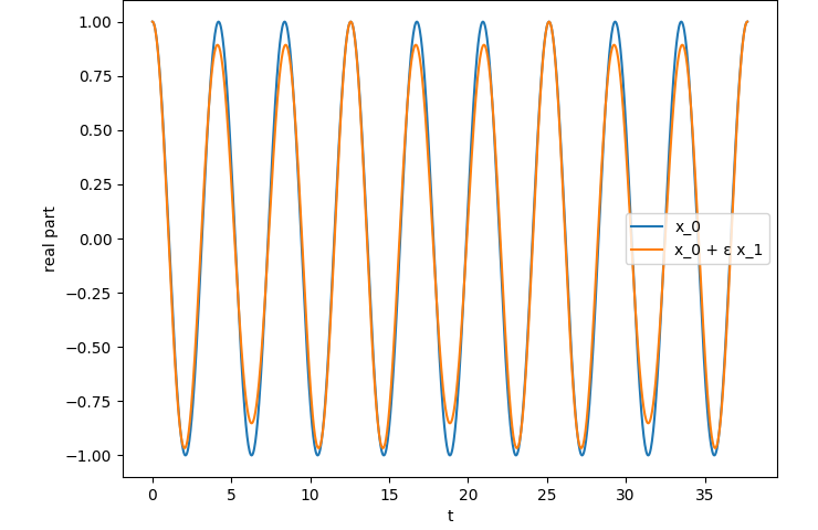
For an arbitrary potential minimum, work out the form of the lowest-order correction to simple undamped unforced harmonic motion.

First we add a small quadratic term to the harmonic oscillator ODE.

$m \ddot{x} + kx + \epsilon x^2 = 0$

Though to push around one less symbol, let’s define $\omega = \sqrt{k / m}$ and absorb a factor of $1/m$ into $\epsilon$ .

$\ddot{x} + \omega^2 x + \epsilon x^2 = 0$

We’ll express our solution as

$x(t) = x_0(t) + \epsilon x_1(t) + \mathcal{O}(\epsilon^2)$

Plugging this into the ODE above, and dropping $\mathcal{O}(\epsilon^2)$ terms, we find that

$\begin{aligned} \ddot{x}_0 + \epsilon \ddot{x}_1 + \omega^2 x_0 + \omega^2 \epsilon x_1 + \epsilon (x_0 + \epsilon x_1)^2 &= 0 \\ \ddot{x}_0 + \epsilon \ddot{x}_1 + \omega^2 x_0 + \omega^2 \epsilon x_1 + \epsilon x_0^2 &= 0 \end{aligned}$

So we recover the original harmonic motion ODE, and gain a second ODE at first order in $\epsilon$ .

$\ddot{x}_0 + \omega^2 x_0 = 0 \\ \ddot{x}_1 + \omega^2 x_1 + x_0^2 = 0$

Again using the ansatz $x_0(t) = e^{rt}$ for the first equation, we find that $r^2 = -\omega^2$ . So the two roots are $r = i \omega$ and $r = -i \omega$ , and the general solution is

$x_0(t) = A e^{i \omega t} + B e^{-i \omega t}$

To simplify the algebra I’m going to assume that $A = 1$ and $B = 0$ , so $x_0(t) = e^{i \omega t}$ . This just amounts to choosing some initial conditions: $x_0(0) = 1$ and $\dot{x}_0(0) = i \omega$ . The second equation becomes

$\ddot{x}_1 + \omega^2 x_1 + e^{i 2 \omega t} = 0$

The general solution is the same as before. For the particular solution, use the ansatz $x_1(t) = C e^{i 2 \omega t}$ .

$-4 \omega^2 C + \omega^2 C + 1 = 0 \\ C = \frac{1}{3 \omega^2}$

$x_1(t) = A e^{i \omega t} + B e^{-i \omega t} + \frac{1}{3 \omega^2} e^{i 2 \omega t}$

Thus our full solution is

$\begin{aligned} x(t) &= x_0(t) + \epsilon x_1(t) \\ &= (\epsilon A + 1) e^{i \omega t} + \epsilon B e^{-i \omega t} + \frac{\epsilon}{3 \omega^2} e^{i 2 \omega t} \end{aligned}$

To facilitate comparison of $x$ and $x_0$ , let’s solve for the same initial conditions we imposed earlier.

$\begin{aligned} 1 &= x(0) \\ &= \epsilon A + 1 + \epsilon B + \frac{\epsilon}{3 \omega^2} \\ B &= -A - \frac{1}{3 \omega^2} \\ i \omega &= \dot{x}(0) \\ &= i \omega (\epsilon A + 1) - i \omega \epsilon ( 1 - A - \frac{1}{3 \omega^2}) + \frac{2 i \epsilon}{3 \omega^2} \\ A &= -\frac{1}{6 \omega^2} - \frac{1}{3 \omega^3} \\ B &= -\frac{1}{6 \omega^2} + \frac{1}{3 \omega^3} \\ x(t) &= \left( 1 - \frac{\epsilon}{3 \omega^3} - \frac{\epsilon}{6 \omega^2} \right) e^{i \omega t} + \left( \frac{\epsilon}{3 \omega^3} - \frac{\epsilon}{6 \omega^2} \right) e^{-i \omega t} + \frac{\epsilon}{3 \omega^2} e^{i 2 t} \end{aligned}$

Now we can compare the two. In this plot $\omega = 1.5$ and $\epsilon = 0.5$ (which is rather large for the model to be quantitatively valid, but qualitatively helps accentuate the difference).

x_0 vs x_1