ODEs

Feb 14, 2020

(3.1)

$m \ddot{x} + \gamma \dot{x} + k x = e^{i\omega t}$

(a) $\gamma = 0$

(b)

$m \ddot{x} + \gamma \dot{x} + k x = 0$

Ansatz: $x = e^{rt}$

$m r^2 e^{rt} + \gamma r e^{rt} + k e^{rt} = 0 \implies \\ e^{rt} (m r^2 + \gamma r + k) = 0 \implies \\ r_{1,2} = \frac{-\gamma \pm \sqrt{\gamma^2 - 4mk}}{2m}$

We have three cases:

$\gamma > 2\sqrt{mk}$ => Overdamped. Will go to steady state without oscillating.
$\gamma = 2\sqrt{mk}$ => Critically-damped. Will return to steady state as quickly as possible.
$\gamma < 2\sqrt{mk}$ => Underdamped. Will overshoot zero faster than critically-damped, and start oscillating.

(c)

$x = Ae^{i\omega t} \\ m = k = 1, \gamma = 0.1 \\ -\omega^2 A e^{i\omega t} + 0.1 i \omega A e^{i \omega t} + A e^{i \omega t} = e^{i \omega t} \implies \\ A (-\omega^2 + 0.1 i \omega + 1) = 1 \implies \\ A = \frac{1}{-\omega^2 + 0.1 i \omega + 1}$

Click here for an interactive Google Colab notebook

import numpy as np
import matplotlib.pyplot as plt
%matplotlib inline

m = 1
k = 1
gamma = 0.1

omega = np.arange(0, np.pi, .001)
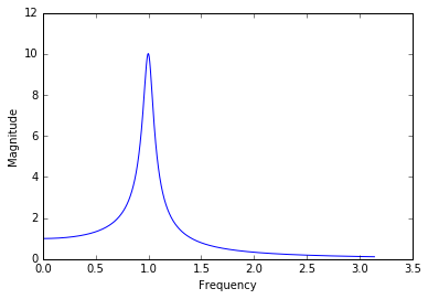
A = 1 / (-m * omega ** 2 + 1j * gamma * omega + k)

plt.plot(omega, np.absolute(A))
plt.ylabel("Magnitude")
plt.xlabel("Frequency")
plt.show()

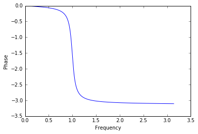
plt.plot(omega, np.angle(A))
plt.ylabel("Phase")
plt.xlabel("Frequency")
plt.show()

(d)

$E = K + U \implies \\ E = \frac{1}{2} m \dot{x}^2 + \frac{1}{2}k x^2 \\$ Try $x = A e^{i\omega t}$

$E = - \frac{1}{2} m \omega^2 A^2 e^{2i\omega t} + \frac{1}{2}k A^2 e^{2i\omega t} \\ E = \frac{A^2 e^{2i\omega t}}{2} (k - m \omega^2)$

Hmmm, to be continued. Useful links: 1, 2

(e)

Useful link: 1

(f)

Not sure what lower order correction means, yet

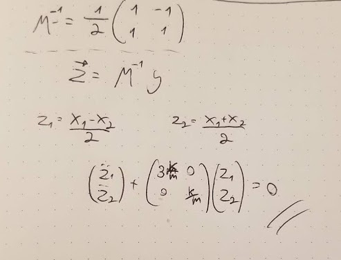
(3.2)

$F = m\ddot{x}\\$

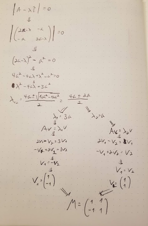
For each particle:

$m\ddot{x_1} = -k x_1 - k (x_1 - x_2) \\ m\ddot{x_2} = -k x_2 - k (x_2 - x_1) \\ \implies \\ m\ddot{x_1} + 2k x_1 - k x_2 = 0 \\ m\ddot{x_2} - k x_1 + 2 k x_2 = 0 \\ \implies \\ m \begin{bmatrix} \ddot{x_1} \\ \ddot{x_2} \end{bmatrix} + \begin{bmatrix} 2k & -k \\ -k & 2k \end{bmatrix} \begin{bmatrix} x_1 \\ x_2 \end{bmatrix} = 0 \\ \implies \\ \begin{bmatrix} \ddot{x_1} \\ \ddot{x_2} \end{bmatrix} + \begin{bmatrix} \frac{2k}{m} & \frac{-k}{m} \\ \frac{-k}{m} & \frac{2k}{m} \end{bmatrix} \begin{bmatrix} x_1 \\ x_2 \end{bmatrix} = 0$

For brevity, denote $a = \frac{k}{m}$

$\begin{bmatrix} \ddot{x_1} \\ \ddot{x_2} \end{bmatrix} + \begin{bmatrix} 2a & -a \\ -a & 2a \end{bmatrix} \begin{bmatrix} x_1 \\ x_2 \end{bmatrix} = 0$

Now, we find the eigenvalues and then eigenvectors so we can eventually get the normal modes:

(3.3)

$y(k) = \alpha y(k-1) + (1-\alpha) x(k)$

Apply two sided z-transform:

$\mathcal{Z}(y(k)) = \mathcal{Z}( \alpha y(k-1)) + \mathcal{Z}((1-\alpha) x(k)) \implies (3.53) \\ Y(k) = \alpha\Big(z^{-1}Y(k) + \underbrace{y(-1)}_{=0} \Big) + (1-\alpha)X(k) \implies \\ \\ Y(k) = (1-\alpha)\frac{z}{z-\alpha} X(k)$

Let’s define $h(k) = \alpha^k \implies \mathcal{Z}(h(k)) = H(k) = \frac{z}{z-\alpha}$ , thus:

$Y(k) = (1-\alpha)H(k) X(k)$

And apply the inverse z-transform:

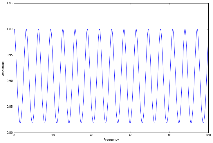
$y(k) = (1-\alpha) \sum_{n=0}^{k} x(n) h(k - n) \\ y(k) = (1-\alpha) \sum_{n=0}^{k} \alpha^{k-n} x(n)$

Now for the frequency response, set $x(k) = exp(i \omega \delta_t k)$ and look at the asymptotic output (3.57):

$y(k) = e^{i \omega \delta_t k} (1 - \alpha) H(e^{i \omega \delta_t}) \\ = e^{i \omega \delta_t k} (1 - \alpha) \frac{e^{i \omega \delta_t}}{e^{i \omega \delta_t}-\alpha} = (1 - \alpha) \frac{e^{i \omega \delta_t (k + 1)}}{e^{i \omega \delta_t}-\alpha}$

Click here for an interactive Google Colab notebook

import numpy as np
import matplotlib.pyplot as plt
%matplotlib inline

alpha = 0.1
k = 100
delta = 1

omega = np.arange(0, 100, .01)
y = ((1 - alpha) * np.exp(1j * omega * delta * (k + 1))) / (np.exp(1j * omega * delta) - alpha)

plt.figure(figsize=(12, 8))
plt.plot(omega, np.absolute(y))
plt.ylabel("Amplitude")
plt.xlabel("Frequency")
plt.show()