Finite Differences: Partial Differential Equations

Week 5

Link to completed assignment

Problem 8.1

(a) Looking at Equation (8.20) in the textbook for inspiration in terms of second order derivatives, we can easily derive the straightforward approximation. $$\frac{\delta^2 u}{\delta t^2} = v^2 \frac{\delta^2 u}{\delta x^2}$$ $$\frac{\delta^2 u}{\delta t^2} = \frac{u_j^{n+1}-2u_j^n+u_j^{n-1}}{(\Delta t)^2}\, ,\quad \frac{\delta^2 u}{\delta x^2} = \frac{u_{j+1}^n-2u_j^n+u_{j-1}^n}{(\Delta x)^2}$$ $$\frac{u_j^{n+1}-2u_j^n+u_j^{n-1}}{(\Delta t)^2} = v^2 \left(\frac{u_{j+1}^n-2u_j^n+u_{j-1}^n}{(\Delta x)^2}\right)$$

(b) We can clearly see that this is a second order approximation in both space and time.

(c) We can substitute Equation (8.9) in for all of our u terms and solve in terms of A to find the mode amplitudes. $$u_j^n=A(k)^n e^{ijk\Delta x} \quad (8.9)$$ $$u_j^{n+1}=2u_j^n-u_j^{n-1}+\frac{v^2(\Delta t^2)}{(\Delta x^2)}\bigl(u_{j+1}^n-2u_j^n+u_{j-1}^n\bigr)$$ $$A^{n+1}e^{ijk\Delta x}=2A^n e^{ijk\Delta x}-A^{n-1}e^{ijk\Delta x}+ \frac{v^2 (\Delta t)^2}{(\Delta x)^2}\bigl(A^n e^{i(j+1)k\Delta x}-2A^n e^{ijk\Delta x}+A^n e^{i(j-1)k\Delta x}\bigr)$$ $$A=2-A^{-1}+\frac{v^2 (\Delta t)^2}{(\Delta x)^2}\bigl(e^{ik\Delta x}-2+e^{-ik\Delta x}\bigr)$$ $$A+A^{-1}=2+\frac{2v^2 (\Delta t)^2}{(\Delta x)^2}\bigl(\cos(k\Delta x)-1\bigr)$$ $$\Bigl(A+A^{-1}=2+\frac{2v^2 (\Delta t)^2}{(\Delta x)^2}\bigl(\cos(k\Delta x)-1\bigr)\Bigr)\cdot A$$ $$A^2-\alpha A +1\, ,\quad \alpha =2+\frac{2v^2 (\Delta t)^2}{(\Delta x)^2}\bigl(\cos(k\Delta x)-1\bigr)$$ $$\frac{-b\pm \sqrt{b^2-4ac}}{2a}\quad \Rightarrow \quad A=\frac{-\alpha \pm \sqrt{\alpha ^2-4}}{2}$$ I am leaving the solution for A in this simplified form.

(d) We know that |A|²=1. Because there are two solutions, A₁ and A₂, we know that A₁*A₂=1. This is only possible if the two solutions are complex conjugates of each other. Therefore, the square root term in the quadratic formula needs to be negative. $$\alpha ^2-4\lt 0$$ $$\alpha ^2 \lt 4$$ $$-2 \lt \alpha \lt 2$$ $$-2 \lt 2+\frac{2v^2 (\Delta t)^2}{(\Delta x)^2}\bigl(\cos(k\Delta x)-1\bigr) \lt 2$$ $$-4 \lt \frac{2v^2 (\Delta t)^2}{(\Delta x)^2}\bigl(\cos(k\Delta x)-1\bigr) \lt 0$$ $$-2 \lt \frac{v^2 (\Delta t)^2}{(\Delta x)^2}\bigl(\cos(k\Delta x)-1\bigr) \lt 0$$ Because the cosine term fluctuates between 0 and 1, the (cos - 1) term will fluctuate between -1 and 0. Thus, $$\frac{v^2 (\Delta t)^2}{(\Delta x)^2} \lt 2$$

(e) Because the real term is the same for both mode amplitudes, they both decay at the same rate.

(f)

(g)

(h)

Problem 8.2

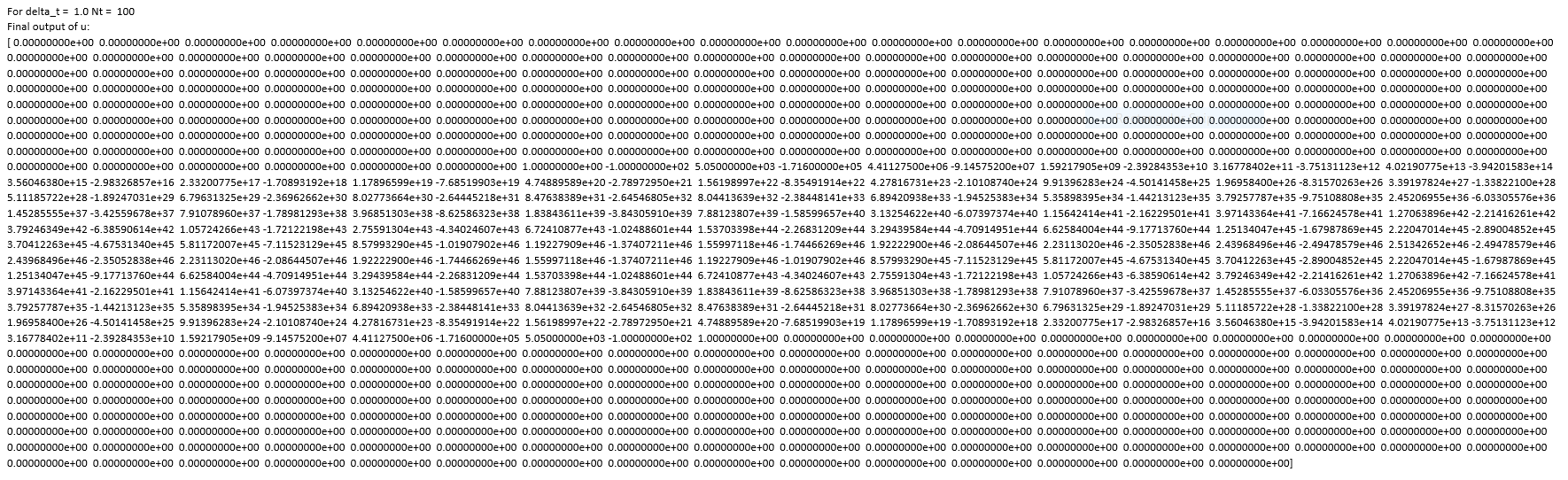
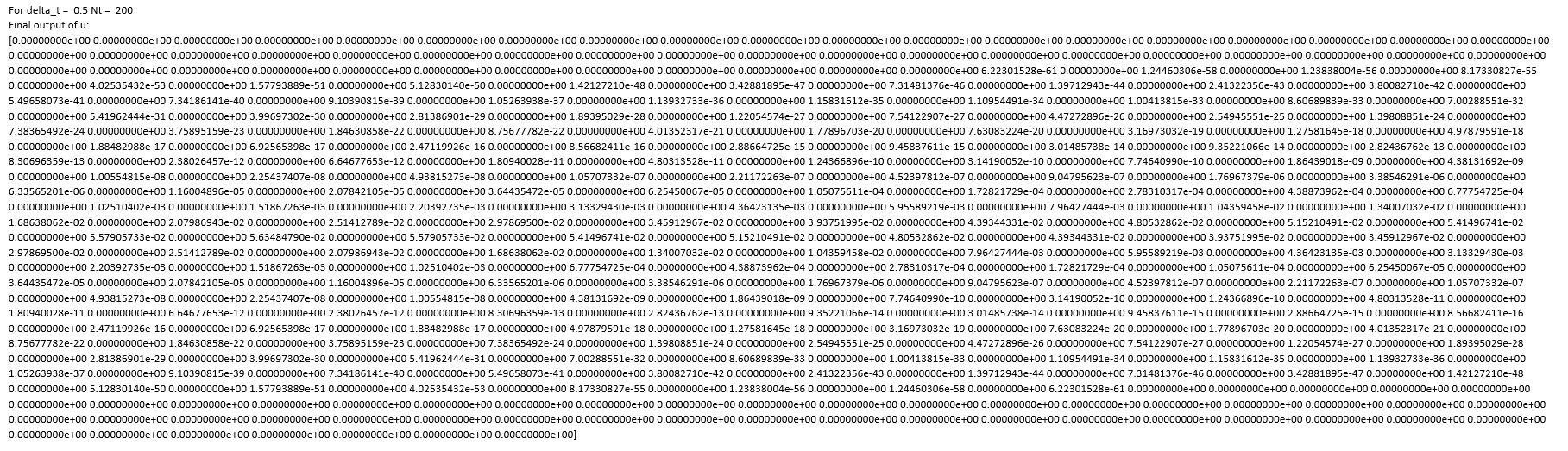
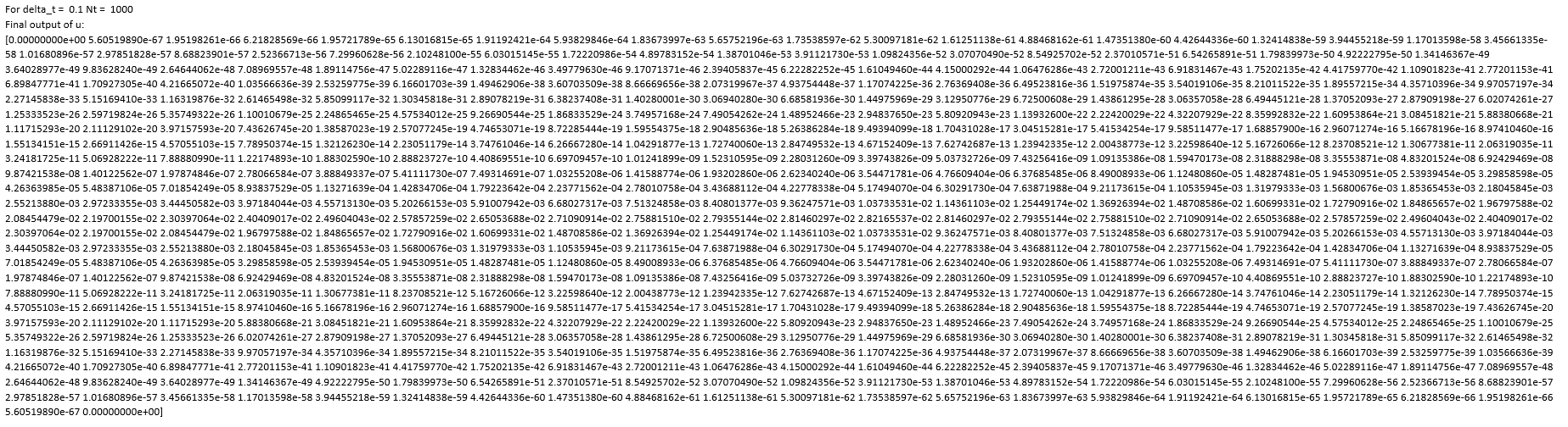
(a) Below is the code for the 1D diffusion problem at different time step sizes of 1, 0.5, and 0.1.

    import matplotlib.pyplot as plt
    import numpy as np

    L = 500
    delta_x = 1.0
    Nx = int(L/delta_x)
    T = 100
    delta_t = [1.0, 0.5, 0.1]

    for del_t in delta_t:
        Nt = int(T/del_t)
        D = delta_x
        x = np.linspace(0, L, Nx+1)    # mesh points in space
        dx = x[1] - x[0]
        t = np.linspace(0, int(T), Nt+1)    # mesh points in time
        dt = t[1] - t[0]
        F = D*dt/dx**2
        u   = np.zeros(Nx+1)           # unknown u at new time level
        u_1 = np.zeros(Nx+1)           # u at the previous time level
        # Set initial condition u(x,0) = I(x)
        u_1[int(len(u)/2)] = 1.0
        print()
        print("For delta_t = ", del_t, "Nt = ", Nt)
        for n in range(0, Nt):
            # Compute u at inner mesh points
            for i in range(1, Nx):
                u[i] = u_1[i] + F*(u_1[i-1] - 2*u_1[i] + u_1[i+1])
            # Insert boundary conditions
            u[0] = 0;  u[Nx] = 0
            # Update u_1 before next step
            u_1[:]= u
        print("Final output of u: ")
        print(u)
    print()
    

The numbers blow up at t = 1, then start to calm down as the step size decreases.

(b)

Problem 8.3

Problem 8.4