Transforms

Week 9

Link to completed assignment

Problem 13.1

In order to prove that the Discrete Fourier Transform is unitary, we need to find the DFT matrix, W. $$W = \frac{1}{\sqrt{N}} \left[\begin{matrix} 1 & 1 & 1 & 1 & \cdots & 1 \\ 1 & \omega & \omega^2 & \omega^3 & \cdots & \omega^{N-1} \\ 1 & \omega^2 & \omega^4 & \omega^6 & \cdots & \omega^{2(N-1)} \\ 1 & \omega^3 & \omega^6 & \omega^9 & \cdots & \omega^{3(N-1)} \\ \vdots & \vdots & \vdots & \vdots & \ddots & \vdots \\ 1 & \omega^{N-1} & \omega^{2(N-1)} & \omega^{3(N-1)} & \cdots & \omega^{(N-1)(N-1)} \\ \end{matrix}\right], \quad \omega = e^{\frac{2 \pi i}{N}} $$ In order to prove that the DFT is unitary, we need to prove that $$WW^\ast=W^\ast W=I$$ We will look at each element W_ij of WW*. $$W_{ij} = \sum_{k=0}^{N-1} \omega^{(j-i)k}$$ Along the diagonal, j - i = 0, so we know that the sum of those values will be N 1's, and $$\bigl(\frac{1}{\sqrt{N}}\bigr)^2(N) = 1$$ So, all values along the diagonal are 1. Now, for the off diagonal values, $$j-i \ne 0, \quad \omega^{j-i} \ne 1$$ Therefore, $$W_{ij} = \sum_{k=0}^{N-1} \omega^k = \frac{1-\omega^N}{1-\omega} = 0$$ because $$\omega^N = (e^\frac{2 \pi i}{N})^N = e^{2 \pi i} = 1$$ All values along the diagonal are 1, and all others are 0, which proves that the DFT is unitary.

Problem 13.2

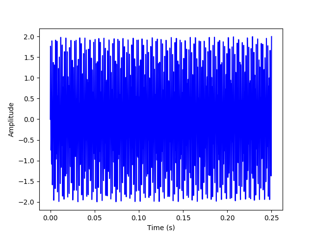
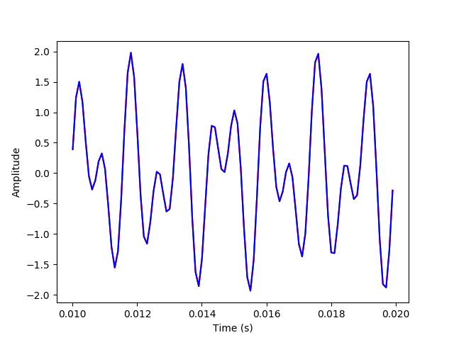
(a) First, we will generate a time series for the sum of two sine waves at 697 and 1209 Hz and plot it, samping it at 10,000 samples per second for 0.25 second.

    import matplotlib
    matplotlib.use('Agg')
    import matplotlib.pyplot as plt
    import numpy as np
    import random

    f1 = 697
    f2 = 1209
    f_s = 10000

    t_tot = 0.25

    N = 2500

    t = np.linspace(0, 0.25, N)

    x1 = np.sin(2*np.pi*f1*t)
    x2 = np.sin(2*np.pi*f2*t)

    x_sum = x1 + x2

    plt.plot(t, x_sum, 'b')
    plt.xlabel("Time (s)")
    plt.ylabel("Amplitude")
    plt.savefig('./plots/transforms/x_sum.png')
    plt.clf()

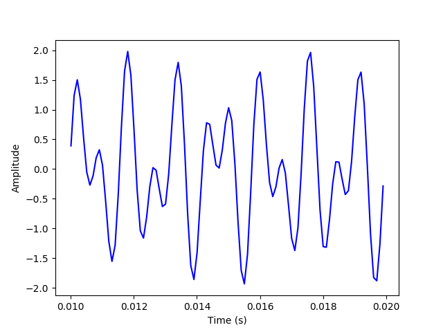
    plt.plot(t[100:200], x_sum[100:200], 'b')
    plt.xlabel("Time (s)")
    plt.ylabel("Amplitude")
    plt.savefig('./plots/transforms/x_sum_zoomed.png')
    plt.clf()
    

(b) Now, we will calculate and plot the DCT for the data, defined by the following equations: $$f_i = \sum_{j=0}^{N-1} D_{ij} t_j$$ $$D_{ij} = \begin{cases} \sqrt{\frac{1}{N}}, \ (i=0) \\[2ex] \sqrt{\frac{2}{N}} cos(\frac{\pi (2j+1)i}{2N}), \ (1 \le i \le N-1) \\[2ex] \end{cases}$$

    D = []

    for i in range(N):
        coef_D = []
        val_D = 0
        for j in range(N):
            if (i == 0):
                val_D = np.sqrt(1/N)
                coef_D.append(val_D)
            else:
                val_D = np.sqrt(2/N)*np.cos((np.pi*(2*j+1)*i)/(2*N))
                coef_D.append(val_D)
        D.append(coef_D)

    f = []

    for i in range(N):
        val_f = 0
        for j in range(N):
            val_f = val_f + D[i][j]*x_sum[j]
        f.append(val_f)

    plt.plot(f, 'b')
    plt.xlabel("Frequency (Hz)")
    plt.ylabel("Amplitude")
    plt.savefig('./plots/transforms/DCT.png')
    plt.clf()
    

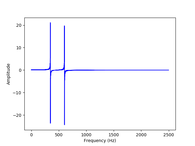
We can see that there are spikes at 348.5 and 604.5 Hz, which are half of the original signal frequencies that are summed together.

(c) Now, we'll get the inverse transform and plot it by inverting D (which is to its transpose in this case), then multiplying D^T and f_i.

      D = np.array(D)
      D_T = D.transpose()
      f = np.array(f)
      x_inv = D_T.dot(f)

      plt.plot(t, x_sum, 'r')
      plt.plot(t, x_inv, 'b')
      plt.xlabel("Time (s)")
      plt.ylabel("Amplitude")
      plt.savefig('./plots/transforms/inv_transform.png')
      plt.clf()

      plt.plot(t[100:200], x_sum[100:200], 'r')
      plt.plot(t[100:200], x_inv[100:200], 'b')
      plt.xlabel("Time (s)")
      plt.ylabel("Amplitude")
      plt.savefig('./plots/transforms/inv_transform_zoomed.png')
      plt.clf()
    

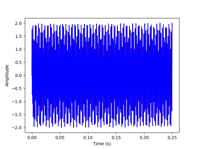
The above plots have the inverse transform signal overlayed on the original signal to verify that they match.

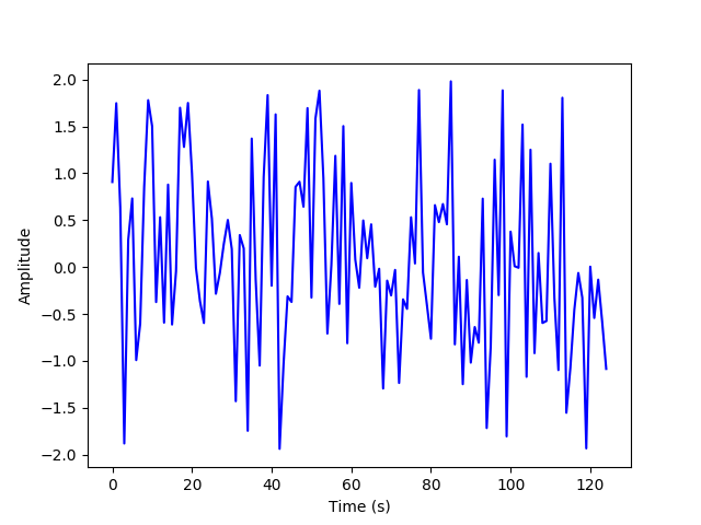
(d) Now, we will randomly sample and plot a subset of 5% of the summed time series.

      M = int(N * 0.05)

      x_rand = random.sample(list(x_sum), M)

      plt.plot(x_rand, 'b')
      plt.xlabel("Time (s)")
      plt.ylabel("Amplitude")
      plt.savefig('./plots/transforms/random_sample.png')
      plt.clf()
    

(e) We will now start with a random guess for the DCT coefficients, and use gradient descent to minimize the error and plot the resulting estimated coefficients.

(f) We will now repeat the gradient descent minimization using the L2 norm and plot the resulting estimated coefficients.

(g) We will now repeat the gradient descent minimization using the L1 norm and plot the resulting estimated coefficients. We will also compare these to the L2 norm estimate, and compare M to the Nyquist sampling limit of twice the highest frequency.

Problem 13.3

We will calculate the inverse wavelet transform, using Daubechies fourth-order coefficients, a vector of length 2¹², with a 1 in the 5th and 30th places and zeros elsewhere. The Daubechies fourth-order coefficients are defined as $$c_0 = \frac{1+\sqrt{3}}{4\sqrt{3}},\ \ c_1 = \frac{3+\sqrt{3}}{4\sqrt{3}}$$ $$c_2 = \frac{3-\sqrt{3}}{4\sqrt{3}},\ \ c_3 = \frac{1-\sqrt{3}}{4\sqrt{3}}$$

      import matplotlib
      matplotlib.use('Agg')
      import matplotlib.pyplot as plt
      import numpy as np

      v_length = 2**12
      v = np.zeros(v_length)
      v[4] = 1
      v[29] = 1

      c0 = (1+np.sqrt(3))/(4*np.sqrt(2))
      c1 = (3+np.sqrt(3))/(4*np.sqrt(2))
      c2 = (3-np.sqrt(3))/(4*np.sqrt(2))
      c3 = (1-np.sqrt(3))/(4*np.sqrt(2))
    

Problem 13.4

(a) A three-component vector x, is made up of x₁ and x₂, which are independently drawn from a Gaussian distribution with zero mean and unit variance, and also x₃, where x₃ = x₁ + x₂. First, we will analytically calculate the covariance matrix of x.

(b) We will now solve for the eigenvalues.

(c) Now, we will numerically verify these results by drawing a data set from the distribution and computing the covariance matrix and eigenvalues.

(d) Finally, we will numerically find the eigenvectors of the covariance matrix, and use them to construct a transformation to a new set of variables y that have a diagonal covariance matrix with no zero eigenvalues. We will verify this on the data set.

Problem 13.5

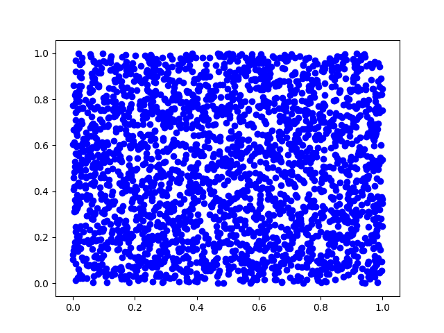
(a) First, we will generate pairs of uniform random variables and plot them.

      import matplotlib
      matplotlib.use('Agg')
      import matplotlib.pyplot as plt
      import numpy as np

      N = 2500

      s1 = np.random.uniform(size=N)
      s2 = np.random.uniform(size=N)

      plt.scatter(s1, s2, c='b')
      plt.savefig('./plots/transforms/13_5.png')
      plt.clf()
    

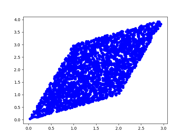
(b) Now, we will mix this data with a square matrix A and plot the result. $$A = \begin{bmatrix} 1 & 2 \\ 3 & 1 \\ \end{bmatrix} $$

      A = np.array([[1,2],[3,1]])
      s = np.array([s1,s2])
      x = A.dot(s)

      plt.scatter(x[0], x[1], c='b')
      plt.savefig('./plots/transforms/13_5_A.png')
      plt.clf()
    

(c) Now, we will make the new data zero mean, diagonalize with unit variance, and plot it.

(d) Finally, we will find the independent components of the data with the log cosh contrast function, and plot it.