
This project is a computational sector of an on-going project that suggests an automatic system for haptic scanning of an object using a generic robotic arm. The goal here is to design a computational scheme for the robot to measure an object by physically probing an object. What can be an alternative way for the robot to engage with the object physically? The suggested scheme can potentially be extended as a system for sculpting an object made out of plastic materials such as clay.
Optic scanners are commonly used for creating
digital copies of (usually freeform) objects.
It is suitable for collecting a large number of
measurement points to sample complex shapes thanks
to its high data rate.
Callieri et al(2004) presented
a system to scan objects adopting a robotic
arm to have accurate control over the scanning process.
However, the limit of creating a digital
twin from optical scanning lies in the fact that it is
a close-ended process, meaning that the 3D model generated from optic
scanning is based on a mesh that contains hundred thousands of points,
which makes it extremely difficult to edit or modify the shape.
scanned mesh of MIT chapel with over 600,000 polygons
Curve interpolation with tangent vectors
Pagani & Scott(2018), Curvature based sampling of curves and surfaces
Since we do not have any information about the object in advance,
we should implement a posteriori approach in planning the toolpath.
Main challenge here is to mathematically define the logic in order
to effectively reconstruct the object digitally.

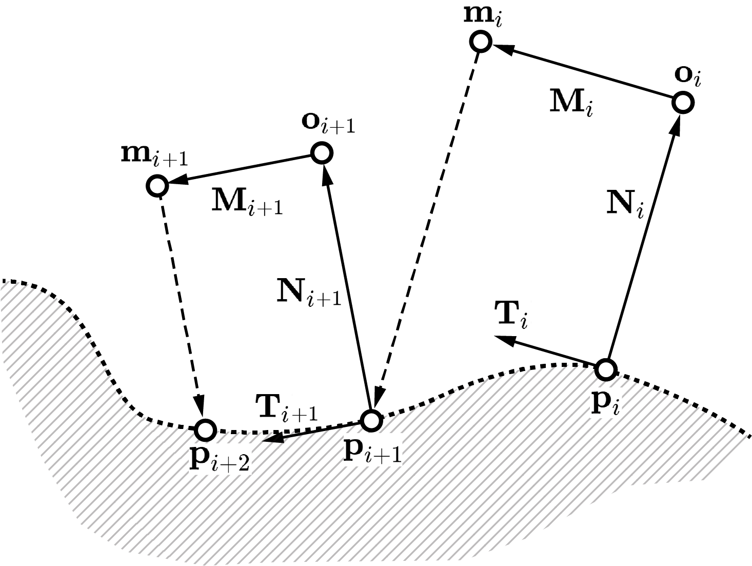
The toolpath consists of five steps:
1. Approach
until the mean value
of distance sensors drops below the critical distance
2. Align
until three distance values normalize in an error range
3. Probe
until the force sensor value reaches the limit value F, then send the point
coordinate and the normal vector data to the master computer
4. Retreat
move for the predetermined value Dr in the direction
opposite from probing
5. Proceed
move for the predetermined
value Dp in the direction perpendicular to the retreat path.
Step 1 to 5 repeat until the distance value jumps abruptly
(when it meets the edge of the flat object) or the probing
tip is in proximity to the first point (when the object is circular).
But here, I will assume that the object is volumetric, which can be described
in a series of periodic curves. Also, step 3 is skipped for now.
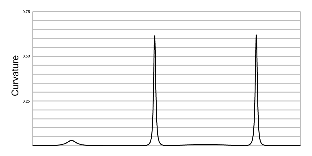
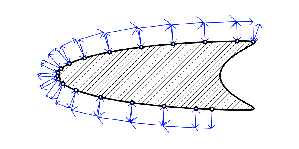
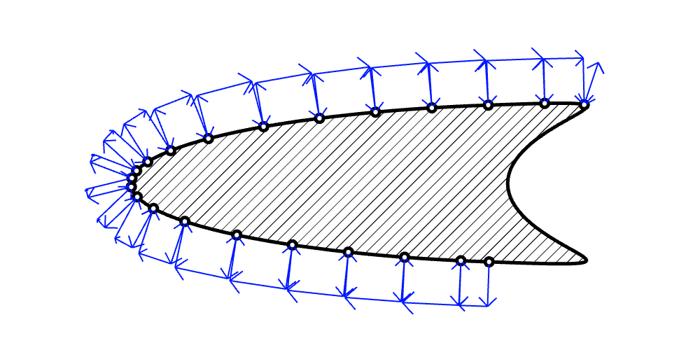
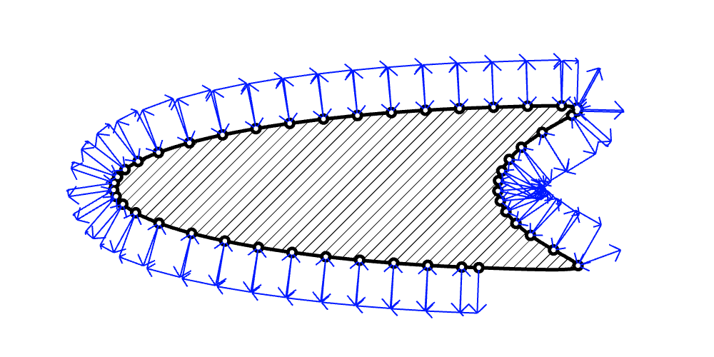
Animation below reveals the potential problem of the scheme that
uses uniform lengths in the iterations. As the shape becomes
sharper, it shows some points where it fails.

When the shape has discontinuity or a sharp change in its curvature,
it is very likely to fail to go full circle. Additional functions should
be added to prevent the toolpath in failing to catch the next probing point.
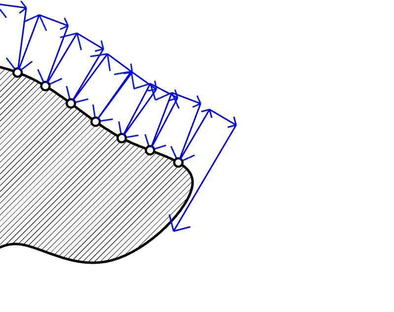
The system should be parameterizing the curve simultaneously as
the robot scan through the surface of the object.
Curvature Based Sampling
Hernández-Mederos & Estrada-Sarlabous (2003) proposed an iterative algorithm
that distributes the control points depending on curvatures.
They introduced a distribution function
\[R(u) = qb(u)+(1-q)l(u) \tag{1}\]
where \(q\) is a filtering parameter in
\([0,1]\), \(b(u) = \int_{0}^{u}\kappa^2(t)dt\) is the bending energy of
the curve, where \(\kappa\) is the curvature. \(l(u)\) is the length of the subcurve until \(u\).
\(q\) is sort of a filtering parameter that can control
uniformity of the points on the curve. Smaller value of \(q\)
gives more uniform length distribution, whereas larger value generates
denser points in the segments of higher curvature.
In this case, curve parameter is discretized, so the funtion \(R\)
is defined in terms of an integer \(i\) instead of \(u\).
Take the derivative of the distribution function
and discretize it, we get
\[{\Delta R} = q\kappa_i^2+(1-q)s_i, \tag{2}\]
where \(s_i = l_i-l_{i-1}\), which is a segment of the curve
between \(i-1\) and \(i\).
Instead of taking the full curve to redistribute the points,
we can use the distibution function (1) for determining the next length
of curve segment.
Since we do not have information
about the shape in advance, I suggest making the \(q\) a
parameter that varies over iterations, as opposed to being a constant
through the scanning. So the function can be rewritten as
\[{\Delta R} = q_i\kappa_i^2+(1-q_i)s_i,\]
where \(q_i\)
It enables the system to "wait" until some amount of data is collected
enough to normalize.
Gradient scheme to control segment length
Using the distance sensor values, the local gradient value can
be computed.
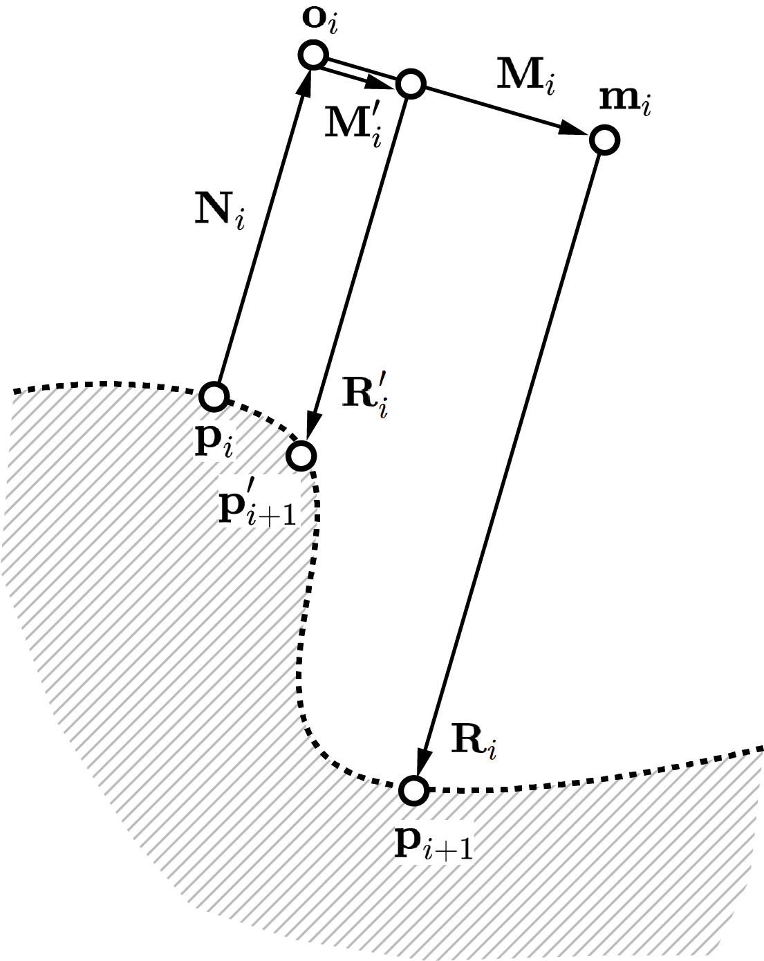
If \(\dfrac{\left|\textbf{R}_i + \textbf{N}_i \right|}{\left| \textbf{M}_i\right|}>\delta_c\),
new vectors \(\textbf{R}_i^\prime\) and \(\textbf{M}_i^\prime\) that satisfies
\(\dfrac{\left|\textbf{R}_i^\prime + \textbf{N}_i \right|}{\left| \textbf{M}_i^\prime\right|}<\delta_c\)
can be substituted.
Hermite Spline
Bezier Spline
Wedge

 Star
Star


3D Scanned Stone


What are the constraints in implementing this? I used
VL53L0X laser distance sensor
for the measurement. Having closer sensing range, I can have higher accuracy
since the farther away from the surface, the higher the error rises.
VL53L0X shows 1.81mm of standard deviation when the distance is 200mm.
Additional constraints might arise when actually using it in the real world.
The first motivation for the project was to make robot physically engage with the project. It is obvious that the next step after the percieving the object is to manipulate the object. Does the hypothesis that "the more concise the computational description of the shape is, easier it is for the designers to modify the shape in the computer, which will then be reflected onto the physical world" still valid?