PIT Final Project

May 17th, 2022

basically an extended problem set on superconducting loops and quantum flux parametron devices

Quantization of Flux around a Superconducting Loop

$$\newcommand{\ket}[1]{\left|{#1}\right\rangle}$$$$\newcommand{\bra}[1]{\left\langle{#1}\right|}$$

Superconductors exhibit long range phase coherence because it's energetically favorable for overlapping cooper pairs to be coherent. Therefore, the wavefunction of a superconductor can be approximated as an ensemble average wavefunction

$$ \psi(\vec r) = |\psi(\vec r)|e^{i\theta(\vec r)} $$

where $\theta(\vec r)$ is a scalar function of the phase of the electron pairs and $\psi(\vec r)$ is typically normalized so that $\psi^*\psi = n_c(\vec r) $ where $n_c(\vec r)$ is the effective density of cooper pairs and can usually be taken to be spatially constant.

The momentum for a single cooper in a weak magnetic field is $$\vec p = m^*\vec v_s + e^*\vec A$$ where $m^* = 2m_e$ and $e^* = 2e$ are the effectie mass and charge of the pair. Extrapolating to all pairs $$ n_c\vec p = n_c (m^*\vec v_s + e^*\vec A) = \bra{\psi}-i\hbar\nabla\ket{\psi}$$ \ $$\bra{\psi}-i\hbar\nabla\ket{\psi} \\ = \bra{\psi}-i\hbar\sqrt{n^*}e^{i\theta(\vec r)} \cdot i\nabla\theta \\ = \bra{\psi}\hbar\nabla\theta\psi \\ = \hbar\nabla\theta\psi^*\psi \\ = n_c\hbar\nabla\theta $$ \ $$ n_c\vec p = n_c\hbar\nabla\theta \\ \vec p = \hbar\nabla\theta = m^*\vec v_s + e^*\vec A $$ and in terms of the superconducting current density and London's penetration depth $$ \vec p = \hbar\nabla\theta = e^*(\Lambda\vec J_s + \vec A) \\ \Lambda = \frac{m^*}{n_ce^{*2}} $$

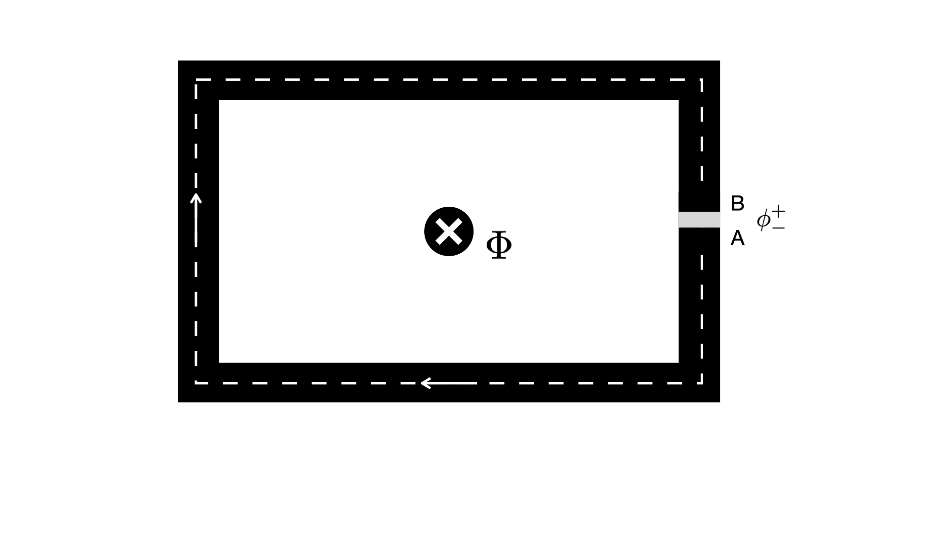
For a supercondcutor with a hole of non-superconducting material, shown in the image below.

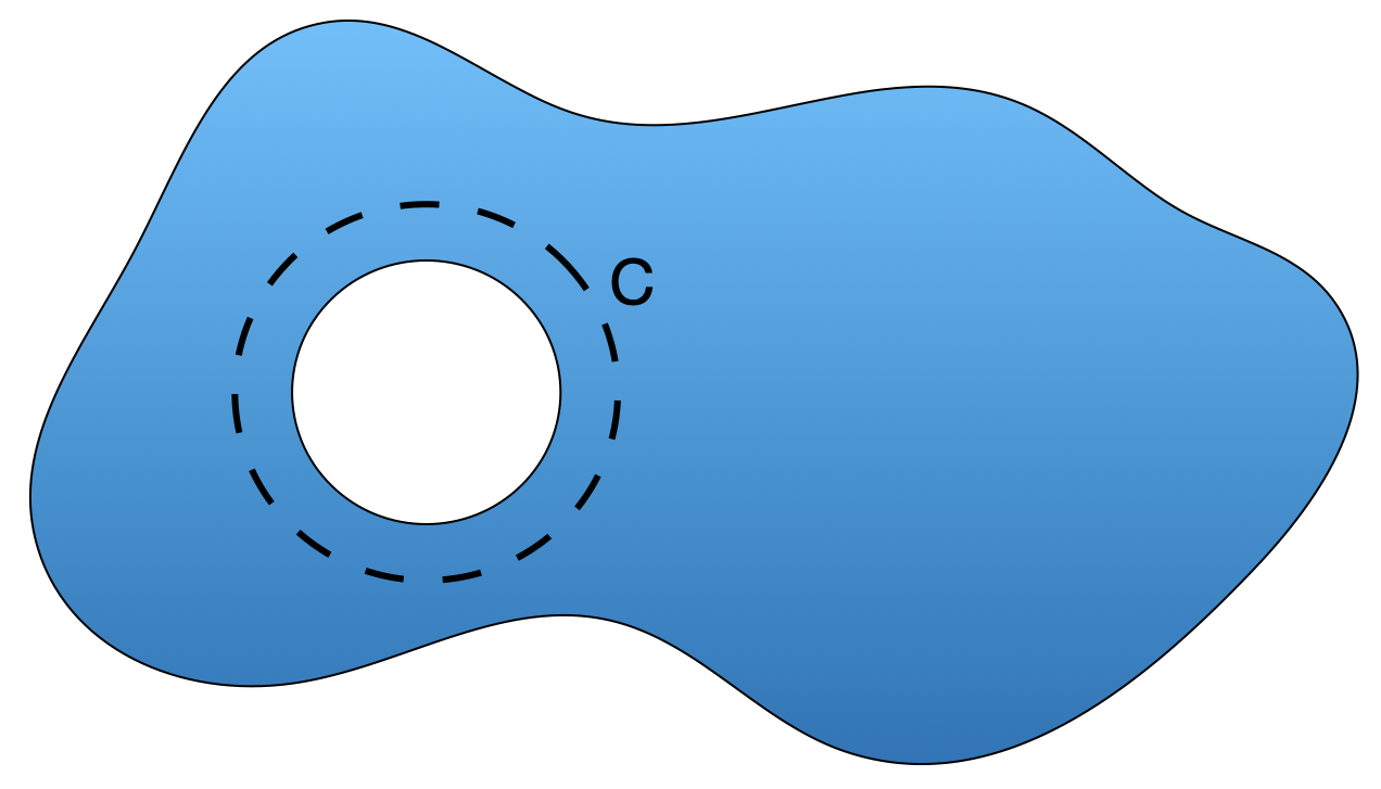
The momentum around the contour C must be $$ \oint\vec p \cdot d\vec l = \hbar\oint\nabla\theta\cdot d\vec l = e_c\oint(\Lambda \vec J_s + \vec A)\cdot d\vec l $$ The closed loop integral across the phase change must be a multiple of $2\pi$ and we'll assume that the contour is deep enough into the material so the current is 0. Then the equation simplies to $$ \hbar 2n\pi = e^*\oint\vec A\cdot d\vec l \\ \hbar 2n\pi = e^*\int_s (\nabla \times\vec A) dS \\ \hbar 2n\pi = e^*\int_s \vec B \cdot d\vec S \\ \hbar 2n\pi = e^* \Phi_s $$ Using Stoke's theorem in the definition of magnetic field, we get an equation for the flux through the non-superconducting loop which is quantized. $$ \Phi_s = \frac{hn}{2e} = n\Phi_0 \qquad n = 0, 1, 2, . . . $$ and $\Phi_0$ is the basic quantum of magnetic flux described by fundamental constants $$ \Phi_0 = \frac{h}{2e} = 2.07\times 10^{-15} \text{Wb} $$

Josephson Junction

TO DO: add some analysis on JJs?

Superconducting Loop with JJ

When a Josephson junction is added to a superconducting loop, there is interference between the wavefunctions across the junction and the flux is generally no longer quantized.

Solve for the phase difference accross the junction by integrating the momentum across the path within the superconducting.

$$ \int^B_A \nabla\theta\cdot d\vec l = \oint\nabla\theta\cdot d\vec l - \int^A_B\nabla\theta\cdot d\vec l \\ = \frac{2e}{\hbar}\oint\vec A\cdot d\vec l - \frac{2e}{\hbar}\int^A_B\vec A\cdot d\vec l $$

Assuming that the loop is deep enough for the current density to be 0. Using Stoke's law as before to convert the integral into a flux, the equation simplifies to $$ 2\pi n + \theta_A - \theta_B = \frac{2\pi\Phi}{\Phi_0} - \frac{2e}{\hbar}\int^A_B\vec A \cdot d\vec l $$

The gauge invariant phase accross a josephson junction is defined as

$$ \phi = \theta_2 - \theta_1 + \frac{2e}{\hbar}\int^2_1\vec A(x, t) \cdot d\vec l $$

Therefore, rearanging the loop gradient, we can find the phase difference accross the loop to be described by $$ \phi = 2\pi n - \frac{2\pi\Phi}{\Phi_0} $$

Then using the Josephson current relation to find the current through the loop $$ I = I_c\sin\phi = I_c\sin\left(2\pi n - \frac{2\pi\Phi}{\Phi_0}\right) \\ I = -I_c\sin\left(\frac{2\pi\Phi}{\Phi_0}\right) $$ The flux through the loop is made up of an externally applied flux, $\Phi_{ext}$, plus the reaction flux produced by the current induced in the loop from the external flux, which can be expressed as the loop inductance times the induced current $$ \Phi = \Phi_{ext} + LI $$ Therefore, we can get the following implicit relation for the current in the loop $$ I = -I_c\sin\left(\frac{2\pi\Phi_{ext}}{\Phi_0} + \frac{\beta_L I}{I_c}\right) \\ \beta_L = \frac{2\pi LI_c}{\Phi_0} $$ and similarly the implicit relation for the flux in a loop, normalized by the flux quantum $$ \frac{\Phi}{\Phi_0} = \frac{\Phi_{ext}}{\Phi_0} - \frac{\beta_L}{2\pi}\sin\left(\frac{2\pi\Phi}{\Phi_0}\right) $$

plotting these:

The flux through the loop oscillates as a function of the changing external flux. When $\beta_L < 1$ there is one possible flux for each external field, but when $\beta_L > 1$ the curves are re-entrant so there is a hysteretic loop between discontinuous transitions - the portions of the curve with negative slope are unstable so as the external flux is varied, the flux through the loop will follow the path with positive slope. This is what is exploited in a RF SQUID Magnetometer: an applied RF field drives the loop through a hysteretic lossy path (each period traps and releases a single flux quanta so the energy dissipation per cycle is $\Phi_0 I_c$), and the amount of RF flux needed to drive the path depends on a quasistatic external flux that is being detected.

This plot also demontrates that the flux in the loop is always equal to the external flux when $\Phi_{ext}/\Phi_0 = n/2$, regardless of $\beta_L$.

The plot above shows the current through the loop for varying external flux and different $\beta_L$. The current always remains less than the critical current in magnitude. And again, the current is re-entrant and nonre-entrant when $\beta_L$ is greater than or less than 1 respectively. The stable states for the current can be found by minimizing the energy of the circuit.

Alternatively, we can think about the superconducting loop and Josephson junction geometry as it's equivalent circuit

And defining a generalized flux angle, which can be described

putting this in WRspice to compare current

Simulating QFP buffer in wrSPICE through pyWRspice

WRspice reminders

pulse(v1 v2 [td tr tf pw per td1 td2 ...]):