HTGAA: Measurement and Imaging
Introduction
Why do we need analytic tools for synthetic projects? The tools for synthetic biology have grown incredibly powerful: DNA synthesis, genome engineering, synthetic cells, directed evolution, cell-free systems, metabolic engineering, and nanomaterial science. However, these tools only cover the second half of the "read/write" cycle. In this class, we will discuss the rationale for developing measurement technologies ("read") to complement these engineering tools ("write"), so that we can understand the effects of our bioengineering efforts and make new products that resemble and/or offer novel functionalities compared to real biological systems.
The lecture will be divided into two sections: First, a theoretical-historical framework for understanding measurement technologies in the life sciences. Second, a review of emerging single cell & spatial sequencing technologies. We will focus predominantly on in situ detection of single molecules (in situ is latin for "in place," referring to detection of molecules in their native spatial arrangement in cells/tissues), including Fluorescent In Situ Sequencing (FISSEQ).
Readings
Required Background & Homework-Related Papers
- The FISSEQ Method: Lee J, Daugharthy E, Scheiman J, Kalhor R, Yang JL, Ferrente TC, Terry R, Jeanty SSF, Li C,Amamoto R, Peters DT, Turczyk BM, Marblestone A, Inverso S, Bernard A, Mali P, Rios X, Aach J, Church GM (2014) Highly multiplexed three-dimensional subcellular transcriptome sequencing in situ. Science 343(6177):1360-3.
- Expansion Microscopy: Chen et al. (2015) Expansion microscopy. Science 347(6221): 543-548
- Theory of RNA and Cellular Molecular State: Kim, Junhyong, and James Eberwine (2010) RNA: state memory and mediator of cellular phenotype. Trends in cell biology 20.6:311-318.
- Foldscope: Cybulski J, Clements J, Prakash M (2014) Foldscope: Origami-based paper microscope. PLoS ONE 9(6): e98781.
Supplement for Foldscope Homework
Supplemental for Lab Homework (TA)
Supplemental Readings on FISSEQ & Spatial Sequencing
- Ginart, Paul, and Arjun Raj (2014) RNA sequencing in situ. Nature biotechnology32.6:543-544.
- Mignardi, Marco, and Mats Nilsson (2014) Fourth-generation sequencing in the cell and the clinic. Genome medicine 6.4:31.
- Avital, Gal, Tamar Hashimshony, and Itai Yanai (2014) Seeing is believing: new methods for in situ single-cell transcriptomics. Genome biology 15.3:110.
Supplemental Readings on Expansion Microscopy and Super-Resolution
- Chen et al. (2016) Nanoscale Imaging of RNA with Expansion Microscopy. Nature Methods 13.8:679–684
- Tillberg et al. (2016) Protein-Retention Expansion Microscopy of Cells and Tissues Labeled Using Standard Fluorescent Proteins and Antibodies Nature Biotechnology 34.9: 987–992
- Chang et al. (2017) Iterative expansion microscopy. Nature Methods 14.6:593–599
- Sydor et al. (2015) Super-Resolution Microscopy: From Single Molecules to Supramolecular Assemblies Trends in Cell Biology25.12:730-748
Supplemental Readings on Theory
- Eberwine, James, and Junhyong Kim (2015) Cellular Deconstruction: Finding Meaning in Individual Cell Variation. Trends in cell biology25.10:569-578.
- Trapnell, Cole (2015) Defining cell types and states with single-cell genomics. Genome research 25.10:1491-1498.
Supplemental Readings on the Historical Context of DNA Sequencing
- Hutchison, Clyde A. (2007) DNA sequencing: bench to bedside and beyond Nucleic acids research 35.18: 6227-6237.
- Goodwin, Sara, John D. McPherson, and W. Richard McCombie. (2016) Coming of age: ten years of next-generation sequencing technologies. Nature Reviews Genetics 17.6: 333-351.
Homework
Hands On Activities (at home):
Part 1: Imaging using FoldScope
This part of the homework is a choose-your-own-adventure in DIY microscopy.
- Assemble your FoldScope and verify its function using one of the included slides. For more resources on FoldScope see https://www.foldscope.com/user-guide
- Explore! We are providing students with several types of living organisms: 1) Spirulina major. A marine cyanobacteria (blue-green algae) culture that contains spiraled trichomes. 2) Hypsibius exemplaris, strain Z151. Tardigrades sometimes known as water bears. You are also encouraged to collect samples from your environment (home, apartment, garden, pet, nearby park, whatever!). The goal is to acquire, using a smartphone, the most beautiful microscopic image you can acquire. Make sure you pay special attention to Focus & Field of view – choose a sample you can get entirely in focus (or not if that’s your artistic whim, but at least achieve a good focus on part of the image). Microscopy is a useful tool in materials science, but since this is a synthetic biology class, please image something biological .
- Collect your experimental results:
- Why did you choose this sample?
- What did you observe?
- What was the final magnification and sampling frequency of your image? (I.e., Approximately how large is each pixel in physical space?) You’ll need to use the final magnification and the sensor size (number of pixels) of your camera to calculate this. Be a good scientist (even though it’s art) and please include a scale bar in your image.
- What is the approximate resolution of your microscope? (Note – this is a harder and more open-ended question than it seems! Please read the FoldScope paper, and supplement on Microscopy.)
- In what ways is FoldScope different from a typical scientific microscope? Discuss at least one difference in optical design. (see supplement on Microscopy)
- Submit your best image(s)!
- Challenge Option: Design & conduct a foldscope experiment with a control and at least one experimental condition. For example, try to incubate your specimen at different temperatures, or exposing them to an environmental challenge.
- What is the hypothesis for how the experimental condition affected the specimen?
- What was the observed result?
Part 2: Design of smFISH / Spatial Sequencing Assay (Computational)
As detailed in the lecture, most in situ RNA measurement technologies are focused on targeted strategies, which use probes to detect one or more RNA targets. For this part of the homework, you will design a FISH or spatial transcriptomics analysis assay. Design of FISH and RNA capture probes is similar to designing PCR probes.
- Choose a problem. As described in the lecture, a “perfect” measurement experiment can mean a lot of things, but in this case, a perfect assay is one that’s well suited to your biological question. So first, you’ll need to think of an RNA imaging application. Describe why imaging measurement is useful for this problem.
- Pick your target genes. What genes would be relevant to this problem? You can choose any number of genes. Here are some typical examples:
- Diagnostic Assay – Pick one or more genes that are relevant to a disease.
- Synthetic Biology – Pick one or more genes that are involved in a synthetic biology circuit or engineering problem. These could be synthetic genes or endogenous genes, depending on the application. Are you engineering an RNA computer? A synthetic organ-on-chip or organoid?
- What is the assay? Would you use multi-color fluorescence? Multiple cycles? Barcoding? Describe why this readout approach is a good fit.
- Pick one gene and design the homology domains (target sequence domains) for 5 probes.
- Download the RNA sequence of your gene from the relevant database (e.g., FASTA from Refseq). Make sure you are using the mRNA sequence (no introns). Depending on how well annotated your organism and target gene is, you may have to manually process the sequence a little.
- Open the Colab Notebook, make a personal copy (File > Save a Copy) and follow the instructions.
- Pick 5 random sequences, each 25 bases long. Use the “Manual Probe Analyzer” section to find the melting temperature and secondary structure of each of your 5 randomly chosen probe sequences. Present the results & discuss – are these probes good? Are they likely to work well together (e.g., bind under the same conditions)?
- Enter the full target gene sequence in the “PROBE-O-MATIC” designer, as well as a target length, thresholds for min/max temperature, and thresholds for min/max secondary structure. Then run the script.
- Play with the settings and run the script several times. Discuss how the probe design problem is constrained, since length, melting temp, and secondary structure can be related. Did you get enough probes? Note, the script output contains all k-mers within the parameters, with the first base number on the target. However, you’ll want non-overlapping probes in your real design, so pay attention to which probes would be overlapping on the target.
- BLAST one of your probes to see how specific it will be to your target. Does it have hits against other genes? If so, what is the melting temperature against the highest off-target hit (NUPACK is good for this using a 2-strand melting model)? Is this a good probe?
Part 3: smFISH Image Analysis (Computational)
Here you will analyze the smFISH images generated by Erkin in the lab experiment.
The experiment was the Fluorescence Multiplex V2 assay on an FFPE pellet of mouse 3T3 cells. The gene panel is a 3 plex of housekeeping genes Polr2A, PPIB and UBC in increasing frequency. These are all expected to be homogeneously expressed in all cells (depending on cell cycle point for each).
Polr2A will be Atto 550, PPIB will be Atto 647 and UBC will be Alexa 488.
- Download & install ImageJ. I prefer the FIJI package https://imagej.net/Fiji
- Download one or more of the Z stack images (nd2 file)
- Import the data: Plugins > Bio-Formats > Bio-Formats Importer & select nd2 file
- In Import Options:
- View stack with: Hyperstack, In Metadata Viewing check the box for Display Metadata.
- Once the image opens, scroll through the metadata fields to find “Nikon Ti2, FilterChanger(EM Wheel1) #x” where X is the channel number. This metadata contains the mapping of channels to gene:
- #1 DAPI – nuclear stain
- #2 FITC – UBC (Alexa 488)
- #3 TRITC – Polr2A (Atto 550)
- #4 CY5 – PPIB (Atto 647)
- Open the display adjustment tool: Image > Adjust > Brightness & Contrast
- Using the sliders on the bottom of the image, scroll through the Z stack (Z) and channels (C)
- Adjust the display settings for each channel. Try adjusting the Min and Max threshold. Try the Auto button. Scroll through Z as you do this. Do not use the “Apply” button, as this will modify the underlying image data, rather than just changing how it is displayed.
- Max project the Z stack – since the sample has some thickness, we can bring everything “into focus” by using a maximum projection on the Z stack. Image > Stack > Z Project. Use “Max Intensity” as the Projection Type.
- Before you try to quantify the data, first visually estimate the number of cells using DAPI and the number of RNA molecules for each gene. Record your best guess estimates. Estimate counts per cell by dividing the number of molecules for each RNA by the number of nuclei.
- Now split the image into each separate channel: Image > Color > Split Channels (the new images files now have a header “C#” for each channel.
- Choose C1 (nuclei) – let’s practice automated segmentation to count the cells. First, duplicate the image to keep the original. Image > Duplicate
- Now choose the duplicate and Go to Image > Adjust > Threshold
- In the Threshold modal, try sliding the min/max thresholds. It should preview the segmentation. Instead of “Default” try some of the automated threshold algorithms. What provides the best result?
- Choose “Otsu” threshold.
- Adjust the image to make nuclei smoother and remove background: Do the following morphological operations: Process > Binary > Close; Process > Binary > Open
- Since some nuclei are touching, split these apart. Use Process > Binary > Watershed.
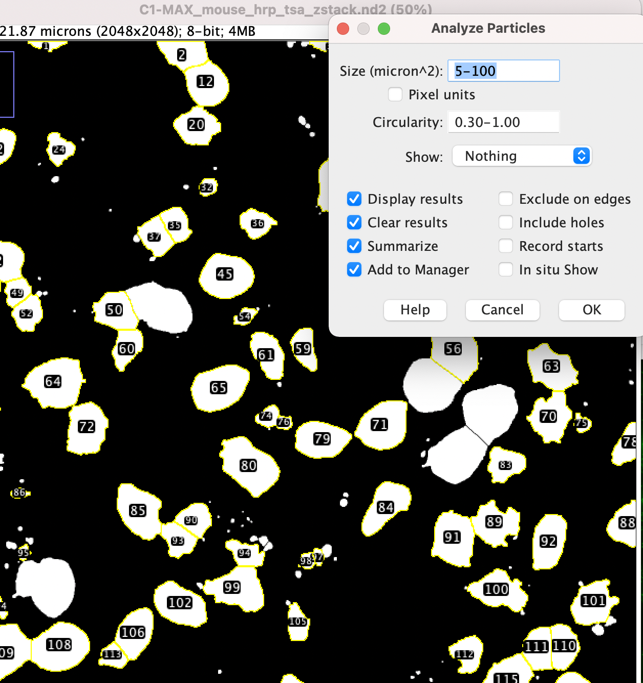
- Now it’s time to analyze the particles. Use Analyze > Analyze Particles.
- Adjust the Size and Circularity setting. For “Show:” choose “Nothing” and check all boxes on the left side (Display Results, Clear Results, Summarize, Add to Manager) then choose OK.
- The objects that have been identified will now have numbers overlayed.
- Try running with different settings until it looks like you’re counting good cells but not noise.
- From the windows that have popped up, choose “Results” – this has the counts of nuclei found and some properties of these. With the Results window selected, Go to Results > Set Measurements and you can choose which results are shown (note these only appear when you re-run the particle analyzer).
- Compare the processed image to the original (you might have to open the file again if the processing modified the display windows). How good is your estimate? How well did the image processing work? Do you see false positives and false negatives? Are there any patterns to which nuclei worked well and which did not work well?
- Repeat Steps 9-20 for each channel of RNA FISH data. Note, for FISH data the Binary > Open step may eliminate a lot of your found RNA – if so you can skip that step.
How did your image processing results compare to the visual assessment? Were your counts for RNA molecules for each gene correlated with the expected expression level (low > medium > high)?
FIJI is a powerful open-source tool for analyzing image data. Feel free to play around with the tool and explore the other macros and options that are available!
Lab Activity: Single Molecule FISH Experiment (TA)
Thanks to the generous help of ACD, Erkin will conduct a fluorescence single-molecule FISH experiment. You can see how the technology works, and also analyze the resulting image data (Homework Part 3)!