Protein Design: Analyzing Protein Folding and Structure
March 21, 2019
Proteins are the workhorses of the cell, running nearly all of cellular activities. In order to be able to perform a vast array of activity, they need to form a large variety of functional shapes. However, for the sake of simplicity and encoding within the genome, they must also be made of standardized parts. This is accomplished naturally via the use of 20 different amino acids. Each amino acid has a "backbone" that is used to connect them together and a "side chain" which allows the chemical variety necessary to produce different three dimensional structures and functions.
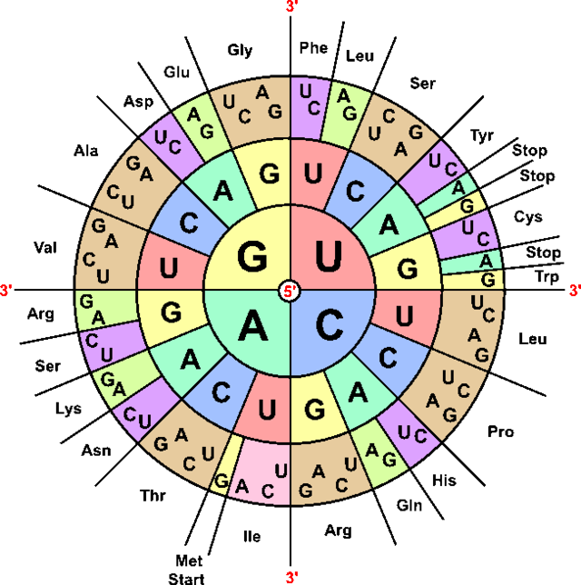
An interesting question to consider is why there are only 20 amino acids that are able to form all of the many functions of proteins. Since each amino acid is encoded by 3 DNA/RNA bases and there are 4 possible bases in each, we could have up to 63 different amino acids encoded (assuming one was used as a stop codon). Scientists have not really found an explicit answer as to why we only have 20, but we can consider some of the potential advantages this system has. The 20 amino acids span a large variety of sizes, polarities, and charges. 2 amino acids are capable of bonding their side chains to form sulfur bridges through the amino acid. It may simply be that the vast majority of potential chemical functions that would be necessary in biology are already accounted for within these 20. Also, having significantly less than 63 amino acids means that the genetic code can have small mutations without necessarily changing an amino acid. Even when an amino acid is changed, it is highly likely that the amino acid shift is to something very similar to the first amino acid. Biology needs genetic variety and mutations in order to create its large variety, and using significantly more amino acids could risk a species long term survival potential due to genetic mutations. Finally, having a repetitive genetic code means that the DNA can mean more than just the protein sequence. Regulation of protein production can rely on the specific genetic sequence, via mRNA folding of the transcript itself, via RNA interfence, via protein bonding to the DNA or the RNA, or via a number of other mechanisms. The repetitive genetic code means that two genes with similar protein sequences can be independently identified and regulated.
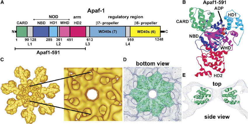
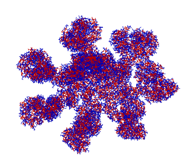
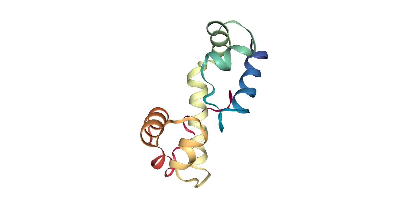
A protein with a particularly interesting three dimensional structure to analyze is APAF1, also known as the "Wheel of Death" protein. This protein is crucial in beginning apopotosis. When bound to cytochrome-C released by the mitochondria, it forms a heptamer in a wheel like structure. APAF1 then binds to procaspase-9, modifies procaspase-9 to caspase-9 (of CRISPR-Cas9 fame), which finally cuts up the DNA to kill the cell. The most frequent amino acid in it is leucine, a nonpolar amino acid, with 139 leucines of 1248 total amino acids (in its largest and most common isoform). According to the NCBI database, there are 10 homologs of APAF1 in humans, chimpanzees, Rhesus monkeys, dogs, cows, mice, rats, chickens, zebrafishes, and frogs, as well as 257 orthologs. This makes sense, as it is a core protein in the apoptosis pathway, necessary in multicellular organisms. It is a part of the family TF323866 on Pfam.
A detailed structure of APAF1 has been solved since 2013, though more recent papers have gotten its structure to the atomic level. It binds with either ATP or DTP (an energy molecule), a heme iron containing group (HEC or HEM), and magnesium in its various structures. Some of the structures also include it bound to procaspase-9. Almost all include it bound to cytochrome-c, as it will only form its wheel structure when bound to cytochrome-c. While it is not included in the SCOP database, it appears to segregate its alpha helices and beta pleated sheets, and would likely be classified as a+b.
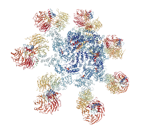
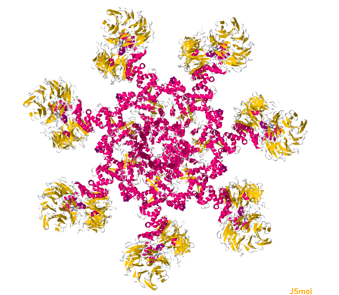
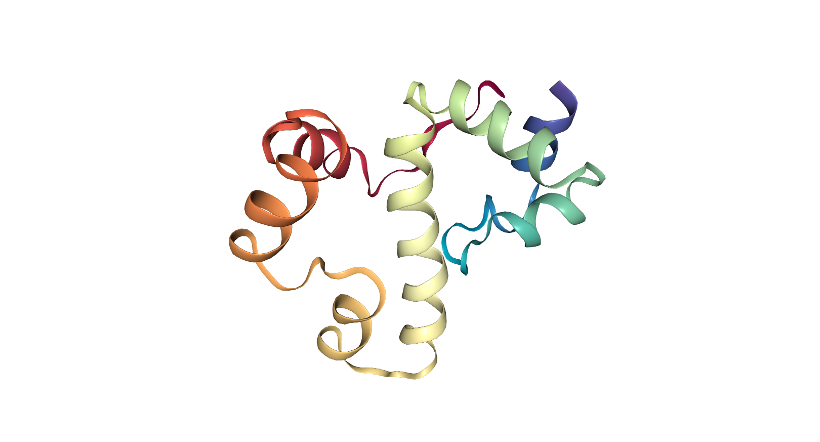
Looking at the visualizations og APAF1, we can see it has slightly more alpha helices than beta pleated sheets, although the areas are highly segregated. It also has its characteristic "wheel" shape, where the outer edges connect to a cytochrome-C and its center binds to procaspase-9.
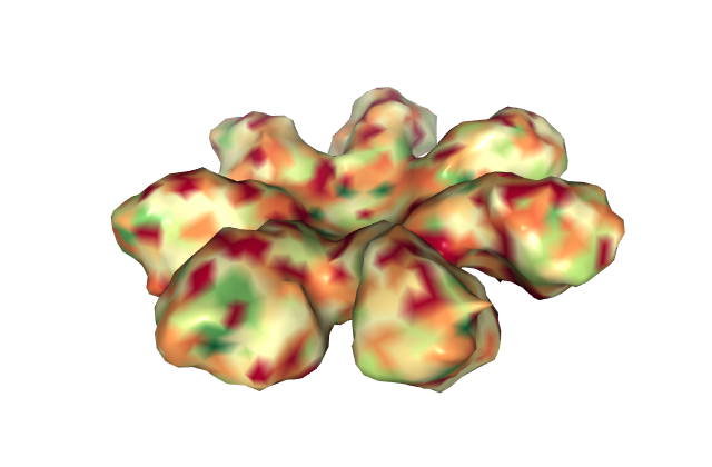
From the visualizations of its hydrophobicity and its surface, we find that it has a large variety of hydrophobicity on its outside. This is likely because it is cytoplasmic and therefore does not need particular hydrophobicity for the membrance. It is more hydrophillic on the outside than its inner barrel, which is more hydrophobic. While its surface does not have any visible binding pockets, the cartoon visualization does show binding at the ends and in the center.
When using PyRosetta, I ran into a number of difficulties; most notably, I had to use Ubuntu for Windows on my computer, and so had to create a separate python file rather than use the Jupyter notebook. The first time I ran the script, something went wrong during this process, as the vast majority of the protein did not fold correctly. Looking into the error output revealed that the fragments of 3 mers and 9 mers had not been read into the file correctly, leading to a lack of information on the secondary structure.
The python script with the questions and answers from the Jupyter notebook is below:
import os
import glob
import shutil
import pandas as pd
#import nglview as ngl
import pyrosetta as prs
prs.init()
from pyrosetta import rosetta
outstr = "\n"
scorefxn_low = prs.create_score_function('score3')
scorefxn_high = prs.get_fa_scorefxn()
native_pose = prs.pose_from_pdb('../../data/1BL0/1BL0_chainA.pdb')
outstr = outstr + "\n" + native_pose.sequence()
DSSP = prs.rosetta.protocols.moves.DsspMover()
DSSP.apply(native_pose) # populates the pose's Pose.secstruct
outstr = outstr + "\n" + 'Native Pose Res 1:' + native_pose.residue(1).__str__()
pose = prs.pose_from_sequence(native_pose.sequence())
test_pose = prs.Pose()
test_pose.assign(pose)
test_pose.pdb_info().name('Linearized Pose')
test_pose.dump_file('outputs/linearized_pose.pdb')
to_centroid = prs.SwitchResidueTypeSetMover('centroid')
to_full_atom = prs.SwitchResidueTypeSetMover('fa_standard')
to_full_atom.apply(test_pose)
outstr = outstr + "\n" + 'Full Atom Score:' + scorefxn_high(test_pose).__str__()
to_centroid.apply(test_pose)
outstr = outstr + "\n" + 'Centroid Score:' + scorefxn_low(test_pose).__str__()
# Q: Visualize the centroid-only structure and see the difference with the full atom that we visualized above?
# Print again the information for the first residue and compare.
test_pose.assign(pose)
to_centroid.apply(test_pose)
test_pose.dump_file('outputs/centroid_only.pdb')
outstr = outstr + 'Centroid Pose Res 1:' + test_pose.residue(1).__str__()
# Loading the files with the pre-computed fragmets
long_frag_filename = '../../data/1BL0/9_fragments.txt'
long_frag_length = 9
short_frag_filename = '../../data/1BL0/3_fragments.txt'
short_frag_length = 3
# Defining parameters of the folding algorithm
long_inserts=5 # How many 9-fragment pieces to insest during the search
short_inserts=10 # How many 3-fragment pieces to insest during the search
kT = 3.0 # Simulated Annealing temperature
cycles = 1000 # How many cycles of Monte Carlo search to run
jobs = 50 # How many trajectories in parallel to compute.
job_output = 'outputs/1BL0/decoy' # The prefix of the filenames to store the results
movemap = prs.MoveMap()
movemap.set_bb(True)
fragset_long = rosetta.core.fragment.ConstantLengthFragSet(long_frag_length, long_frag_filename)
long_frag_mover = rosetta.protocols.simple_moves.ClassicFragmentMover(fragset_long, movemap)
fragset_short = rosetta.core.fragment.ConstantLengthFragSet(short_frag_length, short_frag_filename)
short_frag_mover = rosetta.protocols.simple_moves.ClassicFragmentMover(fragset_short, movemap)
insert_long_frag = prs.RepeatMover(long_frag_mover, long_inserts)
insert_short_frag = prs.RepeatMover(short_frag_mover, short_inserts)
# Q: How many 9-mer and 3-mer fragmets do we have in our database?
# A: We have 200 9-mers and 200 3-mers.
# Making sure the structure is in centroid-only mode for the search
test_pose.assign(pose)
to_centroid.apply(test_pose)
# Defining what sequence of actions to do between each scoring step
folding_mover = prs.SequenceMover()
folding_mover.add_mover(insert_long_frag)
folding_mover.add_mover(insert_short_frag)
mc = prs.MonteCarlo(test_pose, scorefxn_low, kT)
trial = prs.TrialMover(folding_mover, mc)
# Setting up how many cycles of search to do in each trajectory
folding = prs.RepeatMover(trial, cycles)
fast_relax_mover = prs.rosetta.protocols.relax.FastRelax(scorefxn_high)
scores = [0] * (jobs + 1)
scores[0] = scorefxn_low(test_pose)
if os.path.isdir(os.path.dirname(job_output)):
shutil.rmtree(os.path.dirname(job_output), ignore_errors=True)
os.makedirs(os.path.dirname(job_output))
jd = prs.PyJobDistributor(job_output, nstruct=jobs, scorefxn=scorefxn_high)
counter = 0
while not jd.job_complete:
# a. set necessary variables for the new trajectory
# -reload the starting pose
test_pose.assign(pose)
to_centroid.apply(test_pose)
# -change the pose's PDBInfo.name, for the PyMOL_Observer
counter += 1
test_pose.pdb_info().name(job_output + '_' + str(counter))
# -reset the MonteCarlo object (sets lowest_score to that of test_pose)
mc.reset(test_pose)
#### if you create a custom protocol, you may have additional
#### variables to reset, such as kT
#### if you create a custom protocol, this section will most likely
#### change, many protocols exist as single Movers or can be
#### chained together in a sequence (see above) so you need
#### only apply the final Mover
# b. apply the refinement protocol
folding.apply(test_pose)
####
# c. export the lowest scoring decoy structure for this trajectory
# -recover the lowest scoring decoy structure
mc.recover_low(test_pose)
# -store the final score for this trajectory
# -convert the decoy to fullatom
# the sidechain conformations will all be default,
# normally, the decoys would NOT be converted to fullatom before
# writing them to PDB (since a large number of trajectories would
# be considered and their fullatom score are unnecessary)
# here the fullatom mode is reproduced to make the output easier to
# understand and manipulate, PyRosetta can load in PDB files of
# centroid structures, however you must convert to fullatom for
# nearly any other application
to_full_atom.apply(test_pose)
fast_relax_mover.apply(test_pose)
scores[counter] = scorefxn_high(test_pose)
# -output the fullatom decoy structure into a PDB file
jd.output_decoy(test_pose)
# -export the final structure to PyMOL
test_pose.pdb_info().name(job_output + '_' + str(counter) + '_fa')
decoy_poses = [prs.pose_from_pdb(f) for f in glob.glob(job_output + '*.pdb')]
def align_and_get_rmsds(native_pose, decoy_poses):
prs.rosetta.core.pose.full_model_info.make_sure_full_model_info_is_setup(native_pose)
rmsds = []
for p in decoy_poses:
prs.rosetta.core.pose.full_model_info.make_sure_full_model_info_is_setup(p)
rmsds += [prs.rosetta.protocols.stepwise.modeler.align.superimpose_with_stepwise_aligner(native_pose, p)]
return rmsds
rmsds = align_and_get_rmsds(native_pose, decoy_poses)
rmsd_data = []
for i in range(1, len(decoy_poses)): # print out the job scores
rmsd_data.append({'structure': decoy_poses[i].pdb_info().name(),
'rmsd': rmsds[i],
'energy_score': scores[i]})
rmsd_df = pd.DataFrame(rmsd_data)
outstr = outstr + "\n" + rmsd_df.sort_values('rmsd').__str__()
print("\n")
print(outstr)
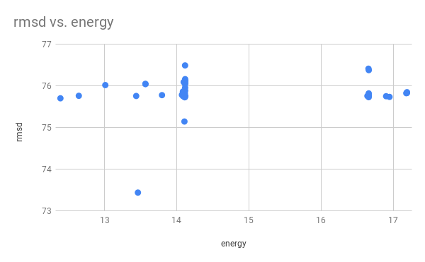
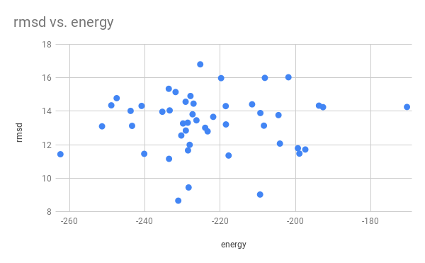
# Q: Plot the energy_score VS rmsd. Are the lowest energy structures the closest to the native one?
# No, the relation between rmsd and energy is not particularly clear.
# This may be due to the algorithm not calculating all of the energy/entropy effects that would exist in the cell.
The output from the above code was the following:
DAITIHSILDWIEDNLESPLSLEKVSERSGYSKWHLQRMFKKETGHSLGQYIRSRKMTEIAQKLKESNEPILYLAERYGFESQQTLTRTFKNYFDVPPHKYRMTNMQGESRFLHPL
Native Pose Res 1:Residue 1: ASP:NtermProteinFull (ASP, D):
Base: ASP
 Properties: POLYMER PROTEIN CANONICAL_AA LOWER_TERMINUS SC_ORBITALS POLAR CHARGED NEGATIVE_CHARGE METALBINDING ALPHA_AA
  L_AA
 Variant types: LOWER_TERMINUS_VARIANT
 Main-chain atoms:  N    CA   C
 Backbone atoms:    N    CA   C    O   1H   2H   3H    HA
 Side-chain atoms:  CB   CG   OD1  OD2 1HB  2HB
Atom Coordinates:
   N  : 0.229, 36.012, 74.172
   CA : 0.041, 35.606, 75.594
   C  : -0.096, 36.849, 76.498
   O  : -0.951, 36.895, 77.382
   CB : 1.225, 34.718, 76.092
   CG : 2.159, 34.156, 74.999
   OD1: 1.688, 33.361, 74.151
   OD2: 3.378, 34.497, 75.007
  1H  : 1.056, 35.74, 73.68
  2H  : -0.43, 35.723, 73.478
  3H  : 0.251, 36.981, 73.928
   HA : -0.884, 35.037, 75.696
  1HB : 1.839, 35.199, 76.854
  2HB : 0.67, 33.892, 76.539
Mirrored relative to coordinates in ResidueType: FALSE

Full Atom Score:46662.2385289
Centroid Score:454.122863078Centroid Pose Res 1:Residue 1: ASP:NtermProteinFull (ASP, D):
Base: ASP
 Properties: POLYMER PROTEIN CANONICAL_AA LOWER_TERMINUS POLAR CHARGED NEGATIVE_CHARGE ALPHA_AA L_AA
 Variant types: LOWER_TERMINUS_VARIANT
 Main-chain atoms:  N    CA   C
 Backbone atoms:    N    CA   C    O    H
 Side-chain atoms:  CB   CEN
Atom Coordinates:
   N  : 0, 0, 0
   CA : 1.458, 0, 0
   C  : 2.00885, 1.42017, 0
   O  : 1.25096, 2.39022, -2.58987e-16
   CB : 1.99452, -0.771871, -1.208
   CEN: 2.35051, -1.69379, -1.45468
   H  : -0.5, -0.433013, -0.75
Mirrored relative to coordinates in ResidueType: FALSE

    energy_score       rmsd                  structure
35   -231.095101   8.653948  outputs/1BL0/decoy_41.pdb
23   -209.375508   9.021131  outputs/1BL0/decoy_30.pdb
12   -228.351223   9.443739  outputs/1BL0/decoy_20.pdb
38   -233.549446  11.155148  outputs/1BL0/decoy_44.pdb
40   -217.730875  11.352236  outputs/1BL0/decoy_46.pdb
4    -262.381694  11.430146  outputs/1BL0/decoy_13.pdb
19   -240.134107  11.453890  outputs/1BL0/decoy_27.pdb
8    -198.935451  11.468517  outputs/1BL0/decoy_17.pdb
43   -228.512963  11.658983  outputs/1BL0/decoy_49.pdb
29   -197.366819  11.712007  outputs/1BL0/decoy_36.pdb
14   -199.338112  11.787165  outputs/1BL0/decoy_22.pdb
48   -228.067943  11.992335   outputs/1BL0/decoy_9.pdb
37   -204.112821  12.066104  outputs/1BL0/decoy_43.pdb
34   -230.291555  12.549900  outputs/1BL0/decoy_40.pdb
30   -223.302879  12.796835  outputs/1BL0/decoy_37.pdb
24   -229.092550  12.844552  outputs/1BL0/decoy_31.pdb
28   -223.952602  13.011182  outputs/1BL0/decoy_35.pdb
13   -251.331840  13.097167  outputs/1BL0/decoy_21.pdb
20   -243.358432  13.125232  outputs/1BL0/decoy_28.pdb
27   -208.356426  13.137354  outputs/1BL0/decoy_34.pdb
36   -218.443369  13.211121  outputs/1BL0/decoy_42.pdb
16   -229.827580  13.268226  outputs/1BL0/decoy_24.pdb
33   -228.583472  13.314477   outputs/1BL0/decoy_4.pdb
1    -226.267214  13.456331  outputs/1BL0/decoy_10.pdb
39   -221.819451  13.663134  outputs/1BL0/decoy_45.pdb
44   -204.486623  13.768157   outputs/1BL0/decoy_5.pdb
10   -227.297727  13.816728  outputs/1BL0/decoy_19.pdb
0    -220.112053  13.845310   outputs/1BL0/decoy_1.pdb
18   -209.300823  13.892698  outputs/1BL0/decoy_26.pdb
11   -235.324900  13.967921   outputs/1BL0/decoy_2.pdb
41   -243.745637  14.020139  outputs/1BL0/decoy_47.pdb
45   -233.379122  14.049248   outputs/1BL0/decoy_6.pdb
42   -192.659804  14.243319  outputs/1BL0/decoy_48.pdb
47   -170.373117  14.254252   outputs/1BL0/decoy_8.pdb
17   -218.493161  14.306151  outputs/1BL0/decoy_25.pdb
25   -240.833522  14.316915  outputs/1BL0/decoy_32.pdb
22   -193.748537  14.333572   outputs/1BL0/decoy_3.pdb
7    -248.869317  14.352598  outputs/1BL0/decoy_16.pdb
21   -211.495260  14.411678  outputs/1BL0/decoy_29.pdb
31   -227.040126  14.453772  outputs/1BL0/decoy_38.pdb
3    -229.143745  14.565474  outputs/1BL0/decoy_12.pdb
46   -247.448064  14.780769   outputs/1BL0/decoy_7.pdb
2    -227.853903  14.909472  outputs/1BL0/decoy_11.pdb
5    -231.810258  15.146400  outputs/1BL0/decoy_14.pdb
9    -233.614844  15.340778  outputs/1BL0/decoy_18.pdb
26   -219.723730  15.978415  outputs/1BL0/decoy_33.pdb
15   -208.108354  15.992851  outputs/1BL0/decoy_23.pdb
32   -201.849057  16.030535  outputs/1BL0/decoy_39.pdb
6    -225.259435  16.802127  outputs/1BL0/decoy_15.pdb