MACHINE WEEK!
This week, my fellow CBA sectionmates and I made an icosahedral robot! It was the one of the highlights of my semester.
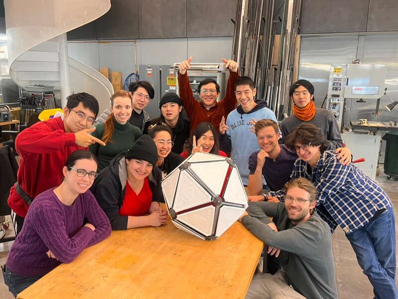
Labububot aka Neilbot 2000 aka Arbitrary Icosahedral Robot
Brainstorm + initial ideation
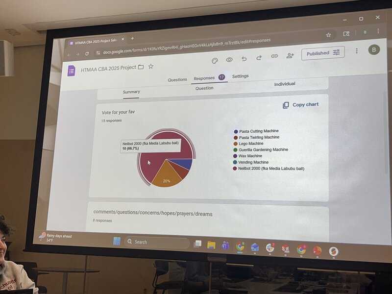
We had a meeting to pitch our ideas, 1 slide each. I pitched the idea with this slide:
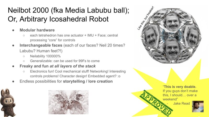
And, the idea won, with 10 of 15 votes!
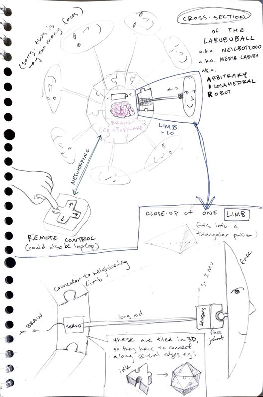
After the meeting I made an organizational Google doc with initial sketches for the robot, places for people to sign up for roles / teams, and logistics for scheduling our first working meeting. Here was my more detailed sketch of the machine:
I signed myself up for the software team.
Icosahedron face numbering
Eitan had helpfully 3D printed a bunch of 20-sided die for each person on our team. We realized that it would be helpful to use this shared reference to create a numbering of the faces of the icosahedron, so we could refer to each individual face and, for example, specify which one(s) to actuate. So the first thing we did was to turn the adjacacency graph of the faces on our 20-sided dice into a .json file. For example, one entry in the map would be
  "1": [
        2,
        5,
        3
      ],
indicating that face number 1 has neighbors 2, 5, and 3 (all faces of an icosahedron are equilateral triangles).
I generated a matplotlib visualization of an arbitrary icosahedron and labelled its faces corresponding to this mapping, which we then double-checked for accuracy to the real dice. I also wanted to plot the face normals, as we would need them later on.
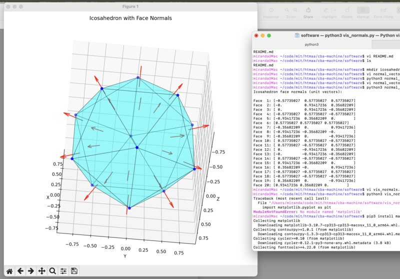
Here
is the code to make this visualization. Please note that I generated
this code using AI, with the prompts:
how do i calculate the normal unit vectors for the middle of the face of an icosahedron
yes, edit the code for a standard icosahedron, and print the normal vectors when i run the script
can you help me visualize these 3d vectors so i can verify them
Calibration math
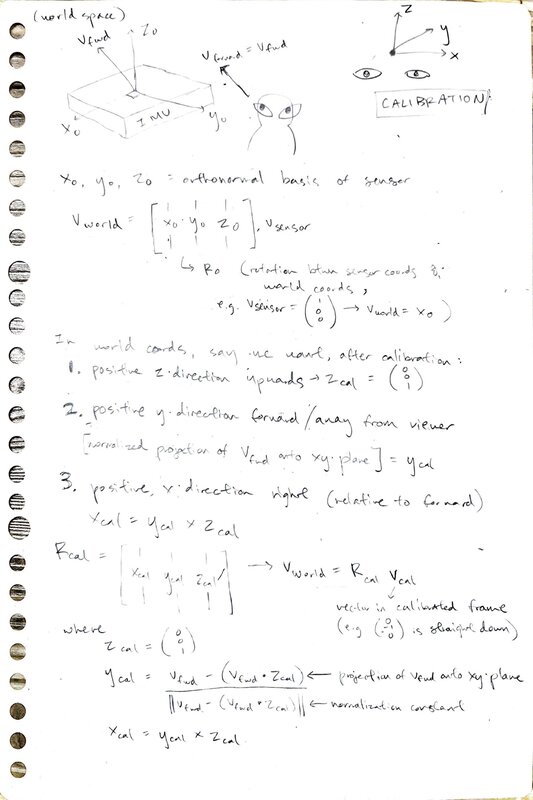
I woke up at 5am in the morning, started thinking about math, and got so excited I couldn’t fall back asleep. I was thinking about how to do calibration, that is – how can we calculate the transform necessary to align the icosahedron (object) frame with the world frame? Without this, we cannot do any kind of meaningful controls – we need to be able to represent the world frame in our simulation so that when we, for example, take a step “forward” (relative to our digital representation of the robot), the robot in fact takes a step “forward” (relative to the real-world robot).
I sketched out my logic for calibration:
And then I quickly coded it up in a Colab notebook.
When I got to lab, I discussed my math with Matti. It was a really interesting conversation – I am coming from a MS in AI, where I had to do many linear algebra proofs, deriving expressions from first principles; Matti is coming from a career in VFX, has not done linear algebra proofs in years, but uses linear algebra very regularly to implement various visual effects. He read my math and said something along the lines of, “Your logic seems right, but I just know from experience that the expression to convert from object to world frame is this, and I can’t prove it to you, but I know it’s right because I’ve been using it for 10 years.”
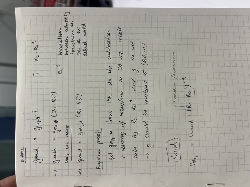
After hours of trying and failing to reconcile our different expressions, we decided to settle it like scientists: with a simple experiment. We would capture readings from the sensor when it is at rest (which we assert to be the same as world frame; that is, we are using the initial readings from the sensor as our basis for the world frame), then rotate it by 90 degrees, and capture readings again. We would compute our calibration matrices (which convert from object to world frame), and in both positions use the calibration matrix to calculate the gravity vector, in world frame. If our calibration is correct, we expect these computed gravity vectors to be similar. Here’s a bit more formalization:
Since we assert that the world frame is the same as the initial object (IMU) frame, we have gworld = gobj, 0(R0R0−1) where R0 is the rotation matrix obtained from the initial quaternion q0 and gobj, 0 is the initial gravity vector from the accelerometer.
After we move the IMU (in this case rotating it by 90 degrees), we should have a consistent gravity vector in the world frame, gworld = gobj, f(RfR0−1) where Rf is the rotation matrix obtained from the final quaternion qf and gobj, f is the gravity vector from the accelerometer, which is in the new object frame (which is no longer the same as the world frame). R0−1 is the inverse of the rotation matrix obtained from the initial quaternion q0 , which represents the translation between the (arbitrary) reference frame of the IMU’s measurements and the real world.
We want to show that gobj, 0(R0R0−1) = gobj, f(RfR0−1), that is, the gravity direction in the world space should always point downwards regardless of which object frame we derive it from.
I tested it in yet another notebook and alas, this math was right. In practice what this means is that at calibration time, we let the IMU settle, and then save the initial quaternion of the IMU at rest (R0). We take the inverse of this, and store this (R0−1) as our “calibration matrix” – this is the rotation which will “undo” the rotation between the IMU and the world space. Whenever we read a new quaternion from the IMU (the robot is in a new position), we multiply it by this matrix to get the quaternion / orientation of the robot in the world frame.
Quaternion reading
Next we wanted to get our nice math hooked up to the real sensor.
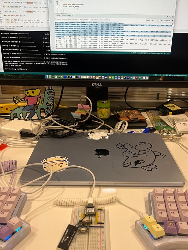
First, I ran some demo code on a breadboard Dimitar mocked up with our IMU, to validate that the sensor works and to get to know the values it outputs.
Then, I Frankensteined two demos – the basic example and the quaternion calculation – into one file which will read the sensor values from the IMU and print them alongside the Quaternion, read-sensor.ino.
In order to use the
quaternion demo code, I had to enable the DMP. On my system, in
Documents/Arduino/libraries/SparkFun_9DoF_IMU_Breakout_-_ICM_20948_-_Arduino_Library/
I found a helpful DMP.md file which explains that “The DMP
enables ultra-low power run-time and background calibration of the
accelerometer, gyroscope, and compass, maintaining optimal performance
of the sensor data for both physical and virtual sensors generated
through sensor fusion. The DMP allows the accelerometer, gyro and
magnetometer data to be combined (fused) so that Quaternion data can be
produced.” All I had to do to enable the DMP was open
Documents/Arduino/libraries/SparkFun_9DoF_IMU_Breakout_-_ICM_20948_-_Arduino_Library/src/util/ICM_20948_C.h
and uncomment line 34, #define ICM_20948_USE_DMP.
With all that done I was able to read the quaternion from the IMU and log it to my Serial Monitor.
UDP -> Bluetooth Low Energy (BLE)
Previously, we were using UDP to connect to the robot over Wifi, but it was a rather convoluted process of asking for the user to type in their IP address to a server we hosted, and then on wake fetching the laptop IP from that site and trying to connect. We also observed that there were some spotty areas around that lab and our connection was generally unreliable. So, we decided to try making the switch to BLE, which ultimately worked super well for our use case.
Matti sent me a MicroPython file for how he had done BLE connection to an ESP32. I converted it to an .ino file using my AI copilot and the prompt “convert @matti_esp32_bt.py into an .ino sketch” – the resulting file was esp32-bt.ino. Then I used the prompt “i want to be able to send commands to my ESP32 over BLE. add a button in @test.html which sends”b” to the ESP32. make some kind of visible acknowledgement that the ESP32 has received it – maybe in @esp32_bt.ino or in the webpage” to create a small test webpage which has a button to send a simple message for BLE testing, test.html. Once validating that this connection works, I wrote a small README for how to run this BLE test.
This code would ultimately become lib-01-ble.ino in our final codebase.
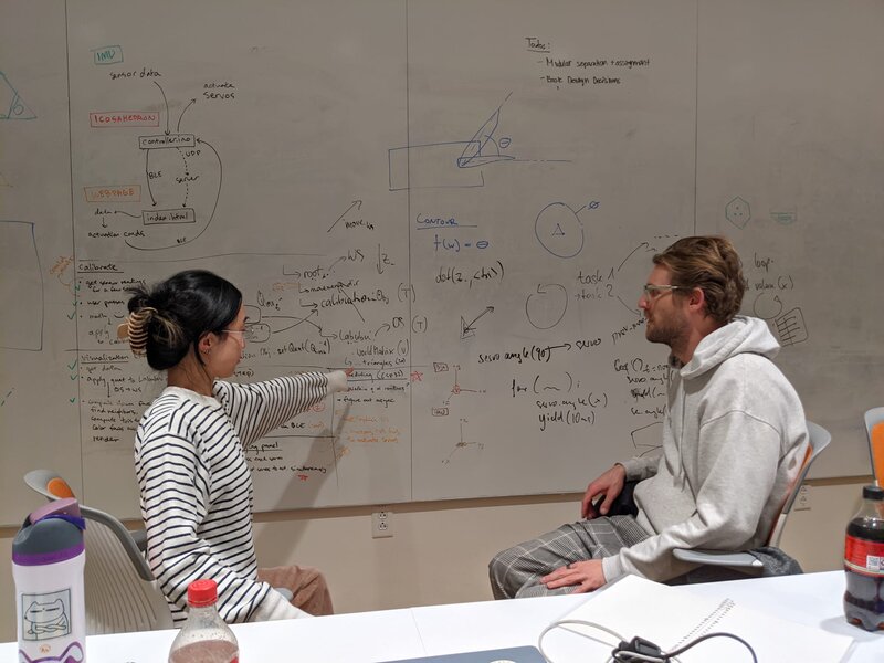
Debugging 3js rotations + calibration with Matti
Next, I moved onto debugging some issues we were having with Matti’s 3js visualization of the icosahedron, in our web controller interface. The IMU data was being read in properly, but several axes were misaligned – the Y and Z axes needed to be swapped, and then the X and Z axes.
Here’s a staged photo of me and Matti discussing where to implement this within the object tree of the 3js visualization.
After an afternoon of fussing I was able to make the fix in brains.js,
in the function updateIMURotationData which returns the new
orientation data for the virtual icosahedron. By updating it here, all
downstream functions pull the correct, axis-flipped orientation of the
robot.
With all that fixed, I experienced the magical moment of being able to rotate my virtual icosahedron using the physical breadboard:
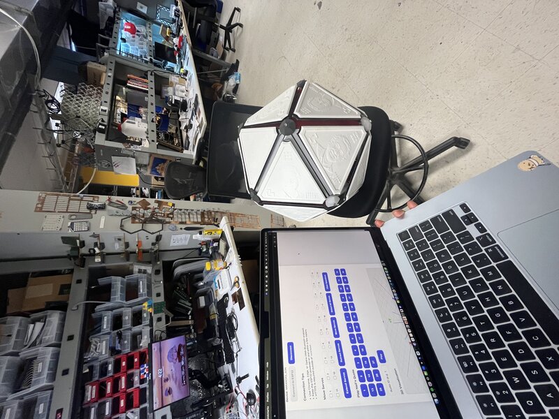
D20 testing & debugging interface
Our next goal was to prepare testing and debugging interfaces so that when the mech team had a working prototype, we could easily verify that e.g. all the servos can be controlled as we expect, we are able to refer to specific face numbers, etc.
To do this I integrated Sophia’s 20-button controller interface into our final codebase, adding Bluetooth functionality and making it call the command for moving the specified servos. Here is the 20-button remote page.
New command protocol
We observe an occasional latency issue with BLE, so to avoid throttling our connection I tried to compress our message from the JSON of strings we were sending into a much more compact, binary encoding, which uses 4 bytes (a 4-bit “command string” and all trailing bytes as data bytes – more info here under Networking / BLE Subsystem). I made sure all the files written up until this point were switched to use the new messaging protocol.
Taking a step
I then implemented the logic to get the robot to “take a step” in brains.js
– since all faces are triangular, the triangular face sitting on the
ground has three neighbors. Based on the desired movement direction we
can compute which of these neighbors we want to roll onto, which we can
do by actuating the other two neighbors. I then pass these two neighbor
indices into a call to move_servo so I can actuate the two
neighbors.
Servo movement
TODO LINK BELOW I debugged the servo library so that
the servos would move to their full rotation. It took a long time for us
to realize that if we specified a servo angle beyond what the servo
could do, it would not move at all. So, we tuned SERVO_MIN and SERVO_MAX
to the specifications of the servo (which Dimitar told us; not sure
where he got them from but I trust him). I added a new file called
servo-params.h to decompose out these constants for code
hygiene.
I also split apart what was previously one “move servo” command into separate “extend” and “retract” commands.
More testing and debugging interface development
I made a bunch of quick modifications to the interface - adding separate buttons to extend and retract the servos in addition to move them (extend, wait a bit, retract); made the movement vector in the visualization a black cone so it would be more obvious, added buttons to allow for the movement vector to be changeable in the 3D visualization, and more; all changes are in the controller index.html. TODO LINK ABOVE
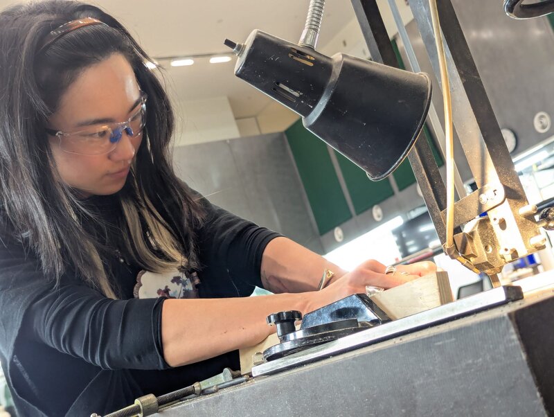
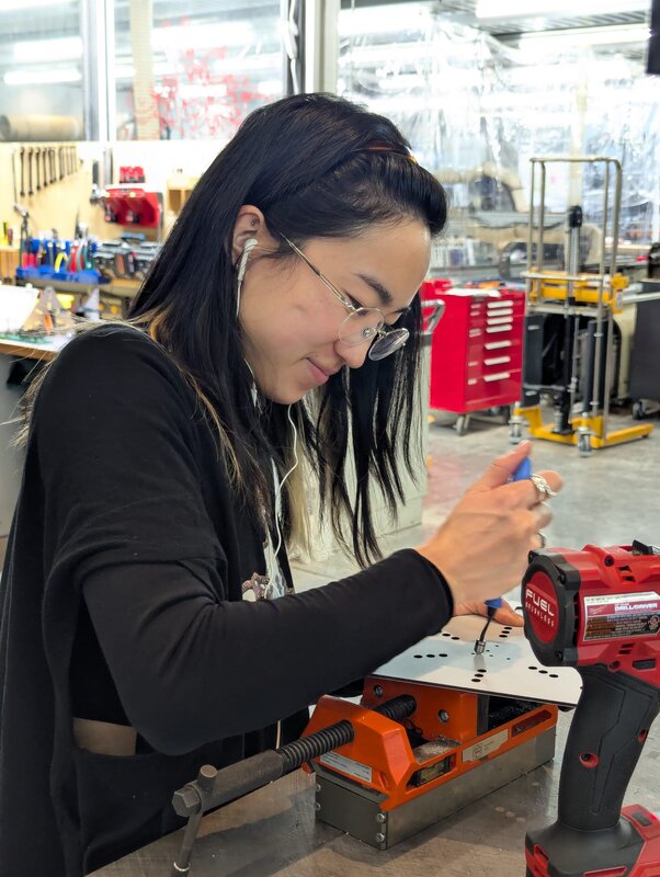
Assembly
At this point, software was way ahead of mech. So as someone with hands I moved on to helping with miscellaneous assembly tasks. I cut some steel rods, cleared some 3D prints for the rack and pinion design, and helped assemble the faces to the actuation mechanisms.
![]()
When most of the robot was assembled, I helped install the limbs by extending the servos so someone else could insert the face into the rack, and then subsequently retracting them back in.
Birth of the Labububot
And then when, the Labububot was assembled and moving, I had to do a bunch of manual changes to accommodate all the small unexpected features of the real robot. For example, I had to flip the extend and retract commands and update the face mapping to correspond to the (arbitrary) order we had assembled the servos.
And eventually, the robot was done!
Death of the Labububot
We filmed our video with me as the puppetmaster – often standing just out of frame, pressing the buttons to make the robot actuate the appropriate limbs for the scene.
And at 5am, the robot attempted – and failed – to take its first steps. The gears ground audibly, and it began to smoke. We hastily turned it off, brought it down to the shop, and disassembled it.
Resurrection of the Labububot
After the dramatic death scene, most of our fellow students went home. But, we knew we’d need to repair the robot to do a live demo in class that same day. Dimitar and I decided to stay and fix the robot, because we figured in our adrenaline-fueled post-all-nighter state we’d still be more productive than after a 3-hour nap anyways.
After some sauter surgery (the closest I’ve felt to being in Grey’s Anatomy)…
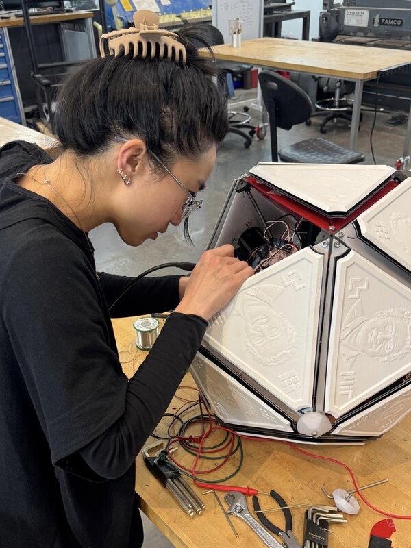
Dimitar and I were able to save the working servos and link them back up to the top hemisphere of the robot.
And, she lived to see the final demo.
What a journey.
The group assignment was The Assignment
Please see our Neilbot page for more details!