03 Random Systems

General Comments

• Doing a lot of floundering in the wilderness.
• My multivariate calculus is still really rusty. Getting better, but it takes me a long time to remember what all the notation means and then how to do things once I understand what the problem is.
• I was short on time this week due to travel and missed class and section, so I'm floundering in the wilderness a little bit blindly and quickly.

7.1 Cumulants

7.2 Coordinate transformations of PDFs

Part (a). Running out of time before class to work these through, but I'm guessing that this is going somewhere clever with the fact that a determinant is basically the area of a paralellogram, justifying why we multiply a PDF by the Jacobian determinant to transform it between coordinate systems

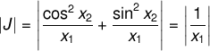
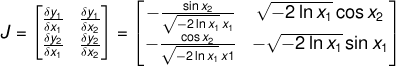
Part (b). p(x₁, x₂) is transformed to p(y₁, y₂) by multiplying by the Jacobian determinant. First we find the Jacobian matrix J:

and from this we can find the Jacobian determinant:

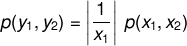
We can now obtain p(y₁, y₂):

7.3 Linear-feedback shift registers

Part (a). The following Python program will print the values of an LFSR of length 4 with the feedback polynomial:

(i.e. taps at bits 4 and 3, indexing from bit 1):

from string import zfill
binstr = lambda x: x>0 and binstr(x>>1) + str(x&1) or ''
bitval = lambda x,n: (x&(1<<n)) >> n

class LFSR4:
    def __init__(self):
        self.x = 1

    def eval(self):
        self.x = ((self.x<<1) | (bitval(self.x, 3) ^ bitval(self.x, 2))) & 0xF
        return self.x

lfsr = LFSR4()
for i in xrange(16):
    x = lfsr.eval()
    print "%02d: %s (%02d)" % (i, zfill(binstr(x),4), x)

The bit sequence produced by this LFSR is as follows, repeating after 15 iterations and not including the state consisting of all zeros, with a flat power spectrum as expected. Decimal values are shown in parentheses.

00: 0010 (02)
01: 0100 (04)
02: 1001 (09)
03: 0011 (03)
04: 0110 (06)
05: 1101 (13)
06: 1010 (10)
07: 0101 (05)
08: 1011 (11)
09: 0111 (07)
10: 1111 (15)
11: 1110 (14)
12: 1100 (12)
13: 1000 (08)
14: 0001 (01)
15: 0010 (02)

Part (b). An LFSR with a clock rate of 1 GHz will require:

Converting to a power of 2:

Since a maximal LFSR will not repeat before iterations, an 92-bit-long LFSR clocked at 1GHz would not repeat in the age of the universe.

7.4 Brownian motion and random walks

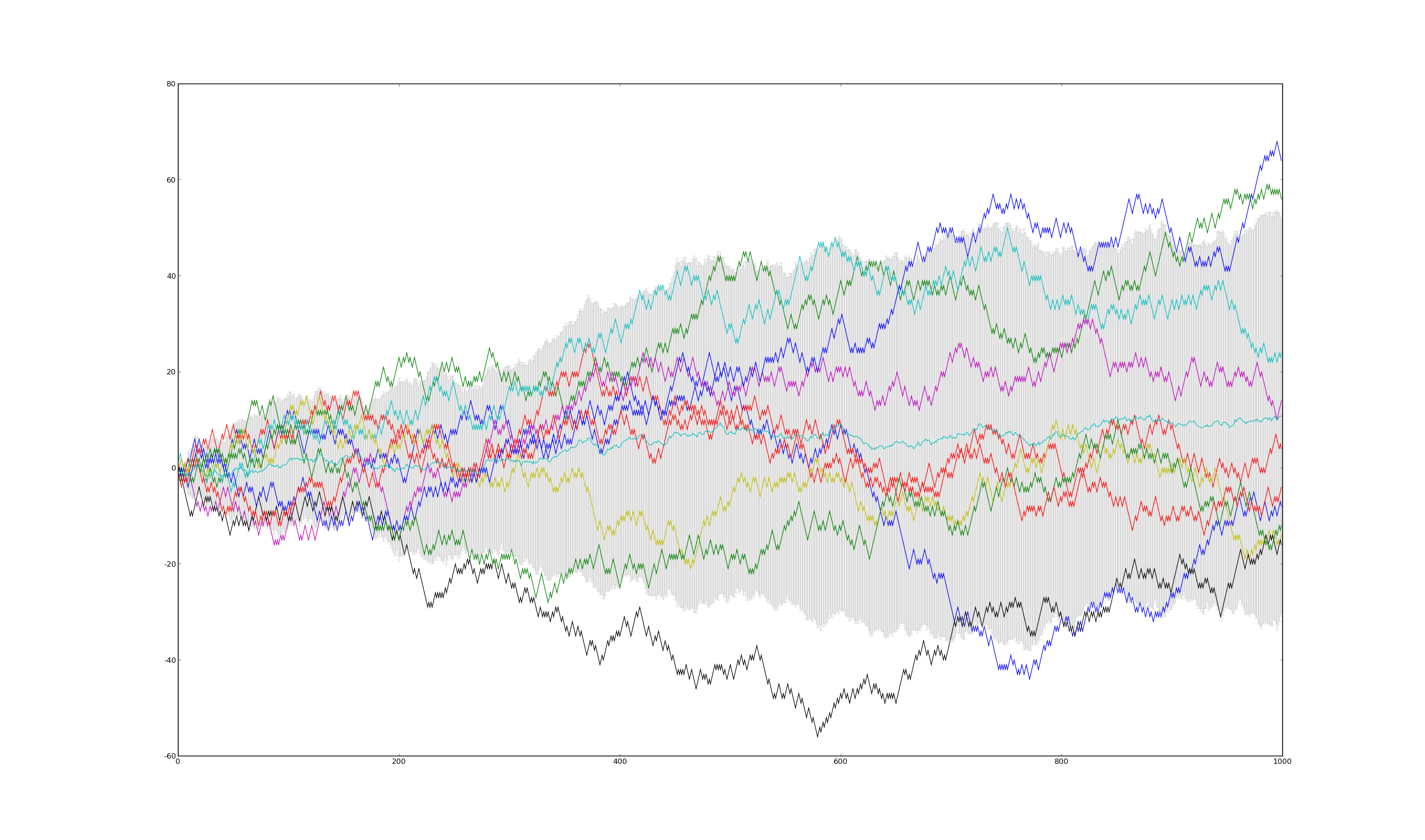
Part (d). Python program: View / Download. The program uses the LSB of a 32-bit LFSR seeded with the 32-bit UNIX timestamp at the time the program to determine the direction at each iteration.

click for much larger version

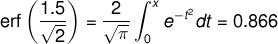
Part (e). Error bars with width 3σ(t) contain the area within 1.5σ(t) of the mean. Assuming that the paths are normally distributed about their mean, the percentage covered by the error bars is:

Therefore, we expect 86.6% of the trajectories to be contained within the error bars.

Return to Index