
The goal of my project was to produce a program that could simulate arbitrary electric field sensor and object geometries and accurately determine the amount of current induced in the receive electrode under a given set of conditions.
There are several different capactive sensing modalities. The one I'm interested in here consists of a driven transmit electrode and a receive electrode. An alternating voltage is applied to the transmit electrode, which induces currents in the receive electrode. The receive electrode is connected to a sensitive transimpedance amplifier that measures this current. As a grounded object is brought near the sensor, the field is changed as the object shunts some of the current to ground. This can be measured at the receive electrode as a decrease in current.
The geometry and voltages of the electrodes and the objects being sensed are known. For the purposes of this project, I am assuming that they are all conductors, and that the environment is free space (the presence of dielectrics in the environment would be a natural extension.)
The core of the problem consists of solving Laplace's equation, given the boundary conditions (the known voltages of the conductors.) Since there are no free charges outside of the conductors, the source term is zero:
where Φ is the scalar electrostatic potential and ∇² is the Laplace operator.
Once the electrostatic potential has been found, the electric field is its gradient:

Once the electric field has been solved, the static charge Qr on the receive electrode due to the electric field can be found:
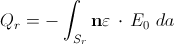
where Sr is the surface of the electrode, and n is the unit vector normal to the surface.
Finally, the current is the time derivative of the charge:

In addition to the mathematical model and solvers, the problem also requires auxiliary functionality to deal with things like representing 3D geometry, and some way to visualize the results. These are ultimately uninteresting in the context of this class, but required a significant amount of work to achieve functionality.
I implemented my simulator in pure C, with no dependencies other than the C standard library. I chose to program in C for efficiency: solving the boundary value problem for the electrostatic potential requires many iterations over a large 3D volume, so optimization of a few key loops is important for reasonable performance.
Originally I intended to use VTK for handling some of the 3D geometry and visualizations, but found it too painful to work with (discussed later.) Rather than sinking more of my time trying to get it to work, I implemented some of the visualization functions using MATLAB's 3D plotting tools.
I originally planned to use STL files to represent the electrode and object geometry, but after failing to find a suitable library to read the files and rasterize them (VTK purports to do this but I couldn't figure it out) I settled on defining all of the geometry programmatically. This is non-ideal from a usability standpoint, as it makes it difficult to use CAD models of sensors and PCBs, but it was a necessary compromise to avoid wasting time on auxiliary functionality and move on with the project.
Implementing a functional representation solver for geometry would have been a useful addition to this project, but that would have been a project in itself.
Most of the computational effort of the simulator goes into solving Laplace's equation for the electrostatic scalar potential. I chose to use the Gauss-Seidel method with successive over-relaxation, which is a compromise between speed and complexity. The solver itself (see solver.c) is relatively simple and the C implementation is able to perform a couple of iterations per second over a 25x25x25 cm grid discretized at 1 mm intervals on a single core on a fast computer. The algorithm is extremely parallel and could be trivially multithreaded (something which I ran out of time to do.) It would also be well-suited to execution on parallel accelerator architectures, such as a GPU or an FPGA. Multigrid methods might yield faster results, but gain complexity and would be less straightforward to parallelize.
To validate the electrostatic potential solver, I first ran the solver by setting a single point at the center of the lattice to a known voltage (simulating a "point conductor" and running the solver. I verified that the results of the solver matched the analytic solution. Unfortunately I didn't save the data from this test and didn't have time to re-run it, so I don't have the plots here.
I also ran the solver on an example geometry and plotted isopotential surfaces for a logarithmic series of voltages, the results of which are shown below:
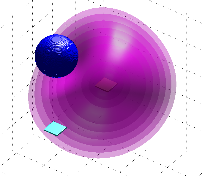
Test geometry and isopotential surfaces. The red electrode is
the transmitter, currently at 100 V. The cyan electrode (held at 0 V by
the analog front end) is the receiver, and the blue ball is a grounded object. The
magenta shells are isopotential surfaces. These plots were generated by
show_geometry.m and isopot.m on the output of the solver.
To evaluate the full simulator, I modeled a simple test geometry similar to one I've worked with before with real sensors. Due to the crude interface for loading models, I've just modeled the electrodes and objects. Since the solver supports arbitrary geometry, it would have been possible with a better interface to fully simulate the entire sensor PCB (in range of the sensor) and the wiring to the electrodes, for a more accurate simulation.
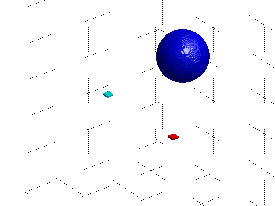
The test geometry consists of two square electrodes, 1cm by 1cm by 3mm. The transmitter is driven to 200 volts peak-to-peak at a frequency of 156.25 kHz (these values are taken from my real sensors.) The receiver electrode is held fixed at 0 volts, and a grounded sphere is brought in range of the setup. The quantity measured is the amount of current induced in the receiver electrode.
I repeated the test for two locations of the test object (the blue sphere.) The first geometry is as follows:
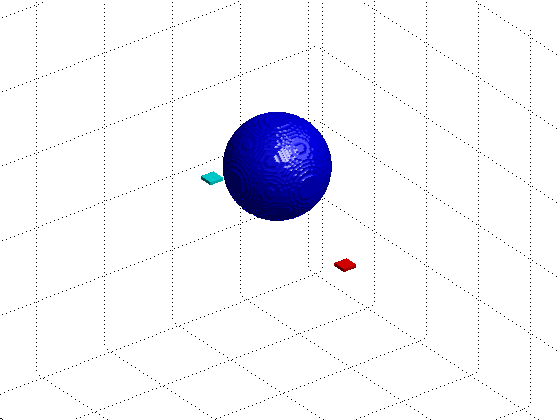
The second geometry moves the test sphere directly above the electrodes, and down closer to the electrodes by a few centimeters:
The results of the complete solver are shown on the plots below. These were generated by solving the electrostatics problem for 32 steps over one period of the transmit waveform, and computing the static charge on the receiver electrode. Given charge over time, I numerically differentiated the charge to find the current.
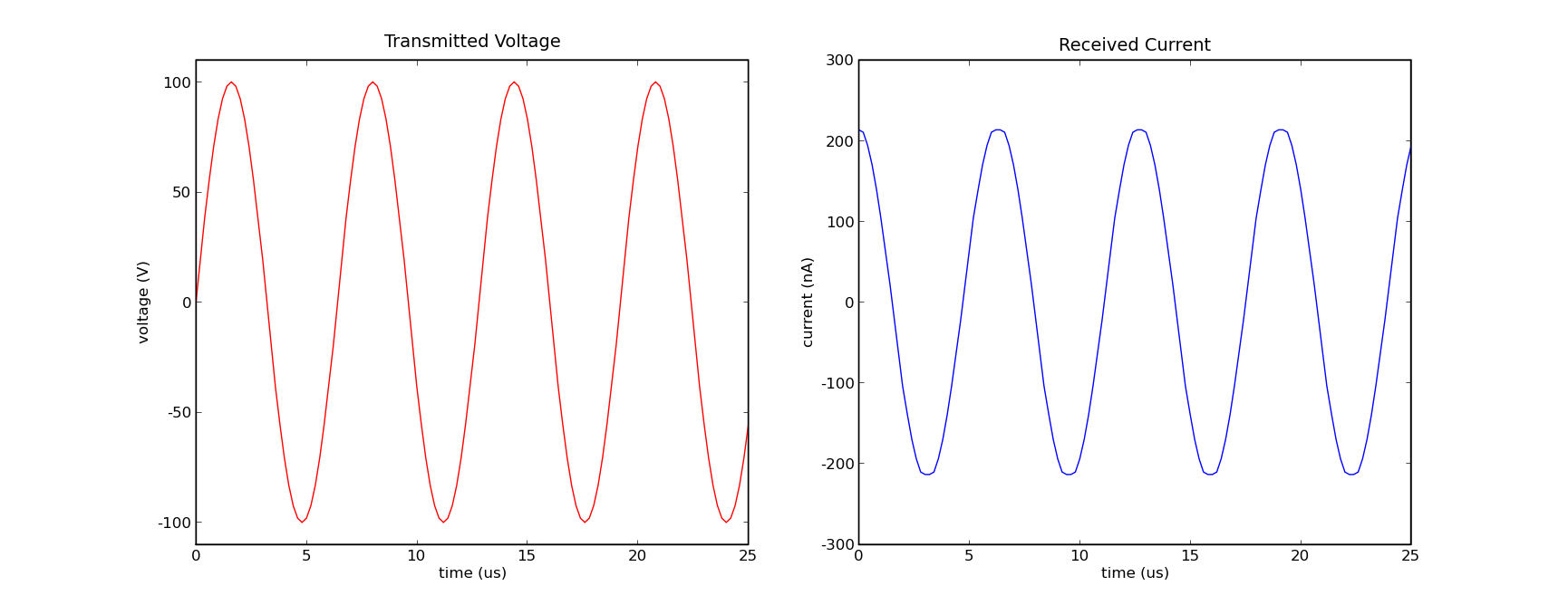
Received current, object far
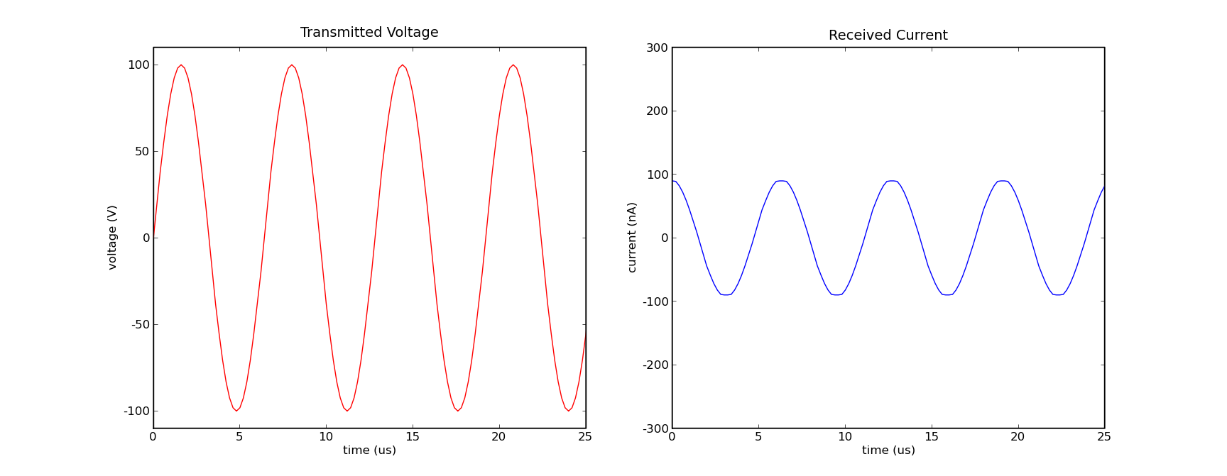
Received current, object near
I ran out of time to actually build and test this sensor geometry with real hardware, but the output is qualitatively correct and the magnitude of the received current is quantitatively reasonable (very close to what I've seen for similar geometries and the response to the presence of the object also matches what I've observed.)
I underestimated the difficulty of working in three dimensions. The amount of data generated can be astounding, and visualizing it to confirm that things are working can be challenging. MATLAB's 3D plotting tools helped, and cutting things into 2D slices and looking at the slices helped as well, but there's no real equivalent to just firing up Python and matlplotlib and taking a quick look at the data like there is in one or two dimensions.
VTK was a huge timesink and a huge letdown for me. I've seen very positive things said about its capabilities and have no reason to doubt that it is indeed quite capable. However, figuring out how to use it left me rather frustrated. The company that makes it has a bit of an odd business model, where they open source the software and sell the documentation as a book and a textbook. Selling a book is fine, but they've left out the middle ground between reading the books cover to cover and becoming an expert in the software, and trying to pick through the API documentation and piece together the functionality you need from a list of classes and function names. The fact that as a company they seem to be very proud of their software engineering techniques and documentation, and many of my frustrations were due to their software engineering techniques (object-oriented code to the excess that it's hard to see the bigger picture in the mess of inheritance diagrams) and their documentation (only as a printed book, more of a tutorial than a reference, covering things like installation and the object-oriented structure in detail while only slightly elaborating on the function names when actually explaining things) was especially maddening.
I'm sure that it's great software, but I'll think twice about trying to use it again unless I'm willing to put a lot of time into learning the whole thing.
Of course, there's never enough time to put into a project like this. The past few weeks have been exceptionally busy with projects and all kinds of things going on. There's plenty of room to push this further. Some of the key things I'd like: