The Nature of Mathematical Modeling - Rachelle Villalon

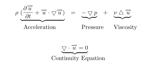
Rules for a Cellular-Space World Predicted by the Navier-Stokes Equations

Abstract
This project is a study of lattice gas techniques for the graphical display of 2-D simulations of fluid dynamics. My motivation behind this project stems from my experience as an architect involved in evaluating building designs represented as digital models brought into software simulation environments to qualitatively understand how daylight or wind theoretically behaves in a building's design. Setting up a simulation environment is typically time intensive and costly, and utmost a luxury as an additional service charged to the client if the design firm carries such resources. By undertaking the study of simulating fluid phenomena, it is my goal to evaluate, understand, and test the advantages and limitations of lattice gas techniques as a math modeling approach for incompressible fluids - ultimately, to help shape an accessible simulation environment for designers with the support of information from an architect's perspective.


  • Exploring Fundamental Questions

    Using the lattice gas method begs the following questions: How does a cellular automaton model lead to the correct form of the Navier-Stokes equations? How does the Navier-Stokes equation depend on the geometry of the lattice? What are the elemental rules for fluid behavior? Asking these questions were necessary for me to understand how something that is traditionally approached by partial differential equations can be represented in a lattice geometry and the rules contained therein.

    Navier-Stokes:

    The Navier-Stokes equations are a set of two differential equations that describes the evolution of a velocity field, u, over time. The first equation describes the motion of fluid through space, along with any forces that act on the fluid. The second equation (continuity) explains that the amount of fluid flowing into a volume must equal the amount of fluid flowing out.


    Cellular Automaton Model for the Navier-Stokes equations


    The following ingredients are needed to yield macroscopic navier-stokes equations on a lattice site (as in the image above), each particle can point to six possible directions with the following parameters:

      1 - A population of particles each moving at the same speed.
      2 - Particles must hop from site to site for a discrete phase space (discrete x, y, and time t)
      3 - A lattice for the particles to travel in. The triangular lattice will be used for this to guarantee isotropic behavior.
      4 - A set of collision rules that define collisions such that particle numbers and momentum are conserved.
      5 - Each particle has a velocity that points to a vertex.

    Essentially, the Navier-Stokes equations are fulfilled in the lattice gas model by particles that behave according to a set of rules that must maintain the laws of conserving mass, momentum, and kinetic energy. The velocities of the particle at each lattice changes according to a collision rule while keeping positions restricted to the lattice site. For a theoretical analysis of how lattice gases recover the Navier Stokes equations, I recommend reading the paper, "Discrete Fluids," as mentioned below.

  • Rules of the Game
  • Keeping the ingredients in mind, the following state table shows some of the scattering rules for fluid simulation. To guide my process, 
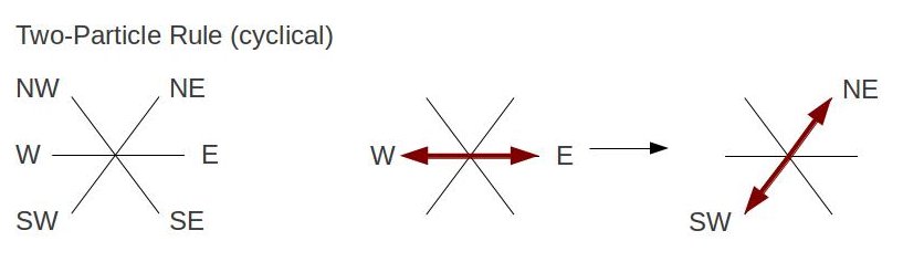
I began by implementing two-particle, three-particle, and four-particle rules described in "Discrete Fluids," a paper written by theoretical physicist Brosl Hasslacher in 1987.


  • Approach using Bit Manipulation for Particle and Lattice Representation
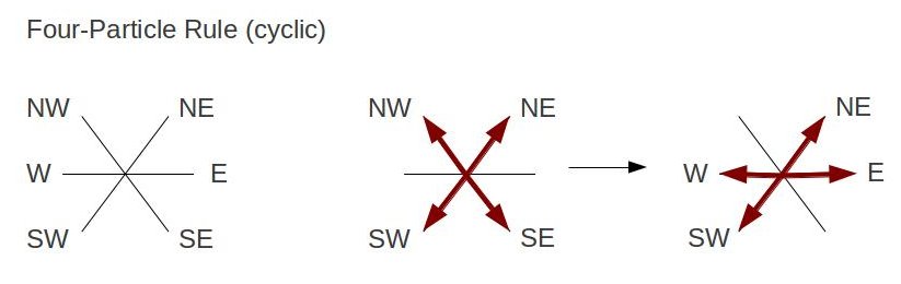
  • The simulation uses bits 0 to 5 to correspond with the six direction paths of a moving particle. In addition, bit 6 represents a rest particle, and bit 7 as a barrier. Each vector (given as ux and uy) is further assigned a coordinate point on the unit circle for travel direction. The following table shows how a vector is mapped to its corresponding direction and binary value.

      Vector 1 = WE = 1 = 00000001
      Vector 2 = SE = 1 = 00000010
      Vector 3 = SW = 4 = 00000100
      Vector 4 = W = 8 = 00001000
      Vector 5 = NW = 16 = 00010000
      Vector 6 = NE = 32 = 00100000
      Vector 7 = Rest = 64 = 01000000
                          Barrier = 128 = 10000000

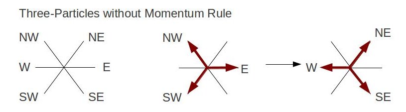
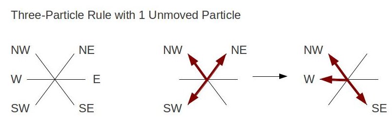
    As mentioned, all moving particles contain the same speed and mass (particle number). Using bitwise OR operators create the collision rules that demonstrate a state changes. For example, if we have one particle moving North-West, another South-West, and the other particle East-bound; the particles state transforms to North-East,South-East, and West respectively. This is shown as rule[NW|SW|E] = NE|W|SE, where NW|SW|E is stored in an array. If a particle runs into a barrier, then the particle reflects off in the opposite direction. This is done by first shifting the NE, NW, W particles (since they have higher value bits) to the right by 3 bits, and then moving SW, SE, WE particles by 3 bits to the left. Once particles move on the lattice, its values are stored in an array called updatedLattice. As particles move again according to the collision rules, its values are then stored to the oldLattice array. Since we've setup a triangular lattice, this means that the sites contain even and odd rows. Moving particles require looping and updating the even and odd rows as separate entities.

    The basic algorithm to simulate fluid flow using a lattice model:

      1. Setup velocities and their representations.
      2. Setup collision rule table that follows the conservation of mass (particle number) and with every rule containing a dual rule.
      3. Set average site velocities vx[i] and vx[i].
      4. Advance the velocity field u.
        4a. Update even sites, apply collision rule.
        4b. Update odd sites, apply collision rule.
      5. If a particle meets a barrier site, then reverse the particle's velocity.
      6. Continue with step 4, looping over the velocity field.

    Using the collision rules and algorithm mentioned, I've setup a lattice site with dimension of 700x400, with 0.2 particle density and speed. The particles are seen moving forward first to their nearest neighbor and then change states according to the collision rule table, the arrows indicate the direction of the particles upon each update step on the lattice.


  • Experimenting with Rules
  • What happens to the simulation when the rules are broken? In other words, what happens if we propose asymmetric particle rules...or disobey the laws of conservation? Architects aren't just interested in seeing how their buildings perform against wind, but they are to an extent, visual artists as well. The idea is to evaluate the genesis of the qualitative outcomes from such a scheme and see the shapes that evolve by creating rules (for design).

    Below are the invented rules describing collision states that break the initial simulation:


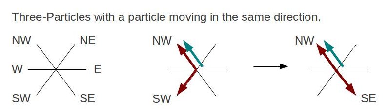
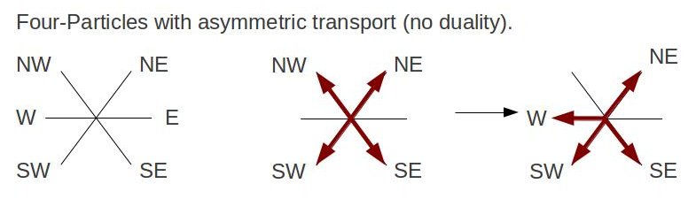
    ...and the accompanying output:


    With the new rules, the qualitative behavior of the navier-stokes equations do not appear to uphold. Particles appear to collectively flow in one main direction. In the previous simulation, we saw that the particles first flow in the direction of their nearest neighbor and scattered according to their respective collision rule.


  • Lessons Learned
    • Using rules to design is not new, George Stiny's "shape grammars" calculates with shapes by using rules - with many rules to choose from that creates an open-ended process.
    • How to make rules on a lattice to approach computing fluid dynamics.
    • A geometric picture of the Navier Stokes equation is a fun way to encode conservation laws.
    • If particles observe conservation laws, then the collisions can create correct macroscopic level behavior.
    • All particles must have the same mass and velocity.
    • Algorithm to simulate fluid flow for triangular lattice gas model.
    • Breaking the rules for particle collision didn't create the random behavior I thought would happen - the particles even appeared to conform to uniform behavior instead.
    • Now that I know how particles move according to the rules given, my next step is to see how particles flow around a barrier such as a building.

  • Problems

    • There are more rules to explore! With many rule combinations, this project touches upon a select few of them for the purpose of qualitatively tracking how particles move in space.
    • For the latter simulation, I would have liked to see how particles behave when moving on a different lattice geometry (circular?).
    • The former simulation creates macroscopic behavior of the Navier Stokes equation by following microscopic behavior of particles on a lattice. The results yielded qualitative information, yet still requires a means to measure quantitative accuracy.

  • Papers that helped along the way:
  • Discrete Fluids

    Data-Parallelism and GPUs for Lattice Gas Fluid Simulations

    Cellular Automaton Models

    The Lattice Gas Model and Lattice Boltzmann Model On Hexagonal Grids

    Lattice BGK Models for Navier-Stokes Equation

    Recovery of the Navier-Stokes equations using a lattice-gas Boltzmann method

    The Classical Lattice-Gas Method

    Real-Time Fluid Dynamics for Games

    Lattice Gas Automata for the Navier-Stokes Equation

    Fluid Flow for the Rest of Us: Tutorial of the Marker and Cell Method in Computer Graphics