For my final project, I asked whether mesh-free field modeling techniques can be implemented using adaptively-sampled distance fields (ASDF), using structural analysis as a test case. In his thesis, Matt Keeter showed how ASDFs could be efficiently used as a geometric modeling data structure. Based on my reading on mesh-free methods, I realized the ASDF contained all the information necessary to directly solve PDEs in place, rather than converting back and forth between a meshed representation. Having a single representation capable of design and simulation would cut down on iteration tmie in design, as well as reduce the errors and manual intervention inherent to geometry conversion.
Most of my research on mesh-free methods lead to the Spatial Automation Lab at UW Madison. Two papers, Finite element analysis in situ and Field modeling with sampled distances, in particular, outline their approaches to implementing Kantorovich's mesh-free method. There is a commercial plug-in for Rhino implementing this called Scan&Solve
These papers showed that it was possible to solve the PDEs for heat and linear elasticity using only signed distance field queries as a geometric primitive. One important distinction from conventional mesh-based FEA, is that the geometric adaptivities of numerical integration and of the shape functions are decoupled.
In planning to adapt these methods to use the heirarchical ASDF, several questions remained. The ASDF stores accurate distances only at the leaf cells and the gradient of the distance field is discontinuous between adjacent leaf cells. Because of this, I'm not certain the generated linear system will behave well. The mesh-free methods only require an approximate distance function, so the remedy to these potential issues will likely be some degree of smoothing between cells.
I started by implementing a 1-d version of the method described by Freytag, et al, following their example of a tensioned cable (the one-dimensional analog to 3D linear elasticity). My Ipython notebook html is here and notebook is here
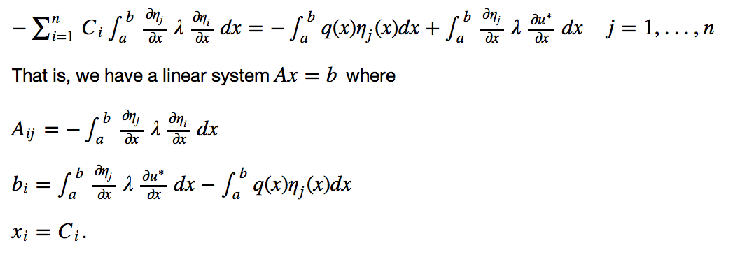
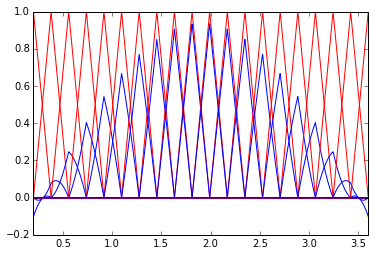
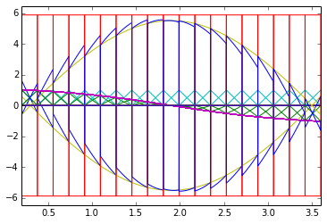
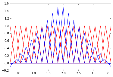
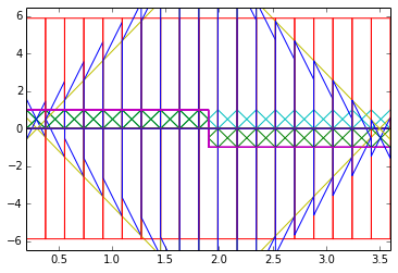
Below I show some plots from this example, used in calculating the quantities making our linear system, shown above. The left image shows the shape functions we allocate, which know nothing about the exact region of integration. We scale them by a function describing distance to the locations where we want to enforce essential (displacement) boundary conditions. The center image shows calculation of derivatives using the chain rule. This requires differentiating the distance function. The right image shows the shape of the cable after solving the linear system, scaling the shape functions by the solution, and adding a boundary condition interpolant.

This was a helpful, complete example to work from, but to do this analysis on a three dimensional ASDF, we need a couple more ingredients. First, we need to be able to numerically integrate shape functions over the complex domain described by the ASDF. Geometrically adaptive numerical integration is tricky to get right, but I found a nice idea based on octrees in this paper. The general idea is to break up the integration domain according to the octree (or in this case, ASDF) description, using adaptive rules to allocate quadrature points over the pieces.
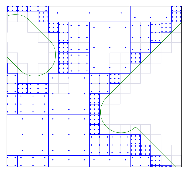
Here we see a part designed and represented as an ASDF. The heirarchical data structure is refined where there is geometric detail, and coarse where the geometry is simple. In the completely filled cells, we can place integration points according to standard Gaussian quadrature rules (shown at the right). In this way, I built up numerical integration routines that use the ADSF infrastructure from Matt's kokopelli project.
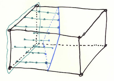
For the leaf cells, we must be more careful to adapt to the boundary. The images below depict the rules we use. If we can find a leaf cell face that is contained in the part, we allocate points across that face by cartesian rules, then fire a ray from each of these points to the intersection with the distance function zero set. We then allocate integration points along these rays.
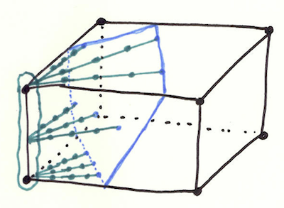
To motivate the other rules, imagine integrating a constant function over a circle. Symbolically, we can choose a cartesian coordinate system or a polar coordinate system and the integrals are equivalent. Numerically, however, there is a big difference, as the polar case converges much faster. With this in mind, we follow the remaining two rules shown above.
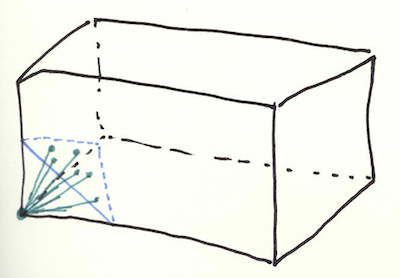
If we cannot find a contained face, but can find a contained edge, we use cylindrical coordinates to lay out the integration points based from that edge. If we can't find an edge, we find a contained vertex and use spherical coordinates based from that vertex.
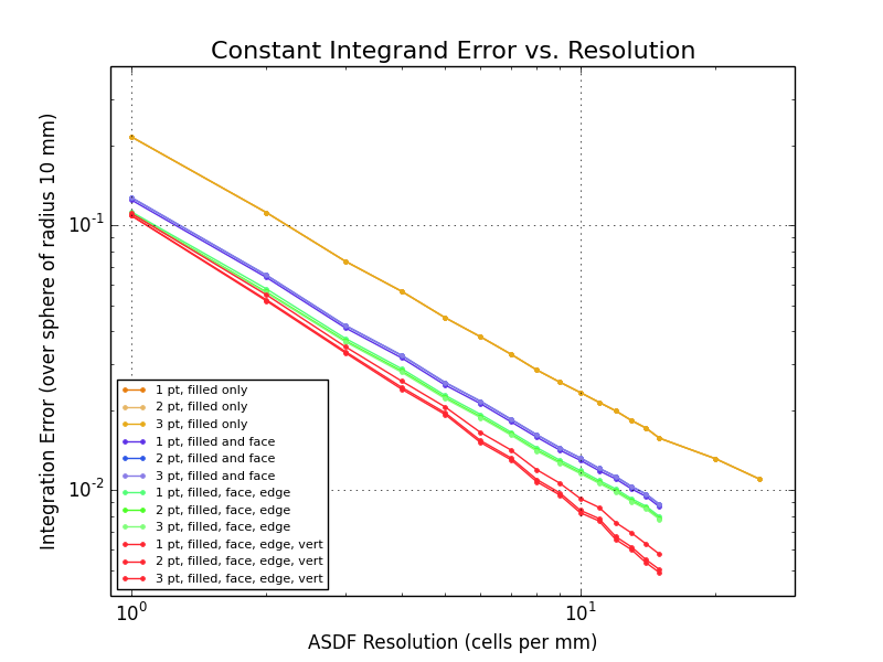
As a test of these rules, we integrate a constant function over a sphere. Since the result should be the volume of the sphere, we can analyze the error of the integration. Above, I'm plotting the pi approximation error vs. resolution while adding each additional leaf cell rule. We see the error when just using the filled cells can be reduced by adding the leaf cell rules. I plot this error for 1-, 2-, and 3-point Gaussian quadrature rules. Since the integrand is a polynomial of order zero (a constant), as expected there is little change as we increase the number of integration points used.
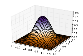
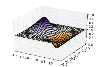
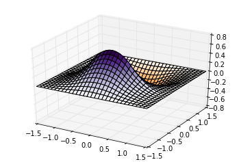
With a heirarchical ASDF numerical integration routine written and testing, I then wrote code for the shape functions I would use to span the solution space. Above, I show a bivariate version of the trivariate B-splines I implemented. On the left is a degree 2 b-spline, and the other two images show the x and y components, respectively, of its gradient. A nice reference on B-splines is this book.
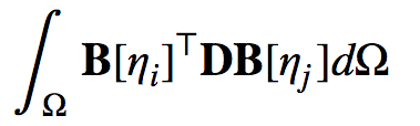
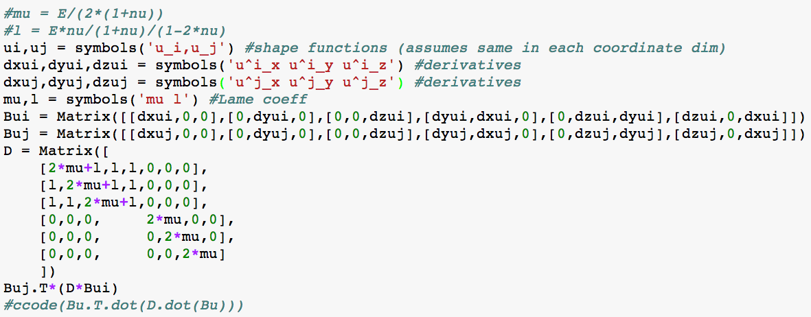
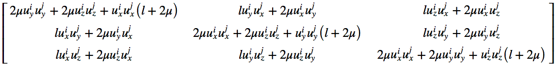
With these B-splines available for use, I then wrote the specific integrals to compute over the geometry. For this, sympy and ipython were very helpful. In particular, sympy has a command called ccode which can generate code to be copied directly into a C source file. To calculate the stiffness matrix entries, we need to manipulate the stress-strain and strain-displacement matrices, calculating their action on the boundary-distance-scaled shape functions. Below are images of the original integral to compute, sympy for symbolic manipulation, an expression for the incremental matrix, and the C code.
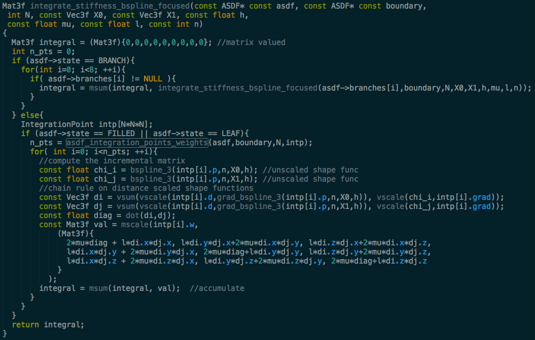
The C routine above is called after we have descended through the ASDF to the smallest cell containing the support of the shape function. The routine then splits until the integral is broken into filled, empty, and leaf cells. For filled and leaf cells, we allocate integration points, and calculate the weighted matrix to add to the running total for the full integral. A similar calculation gives the other terms in the energy balance equation for linear elasticity, accounting for body forces, essential boundary conditions, and traction boundary conditions.
With these routines written, we are ready to test with a full example. Below I show a cylidrical cantilever beam (white), held by a fixed support. For this first test, I just allocated shape functions uniformly across the 3d bounding box of the geometry. The ASDF from the beam generates the structure for integration, and the ADSF from the support generates the distance field by which to scale the shape functions. This resulted in a 2k x 2k linear system to be solved.
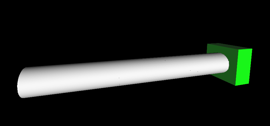
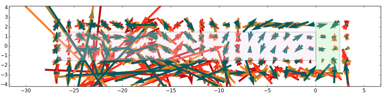
The base of each arrow is a point we've allocated three trivariate B-spline shape functions (one for each spatial dimension. The arrow vector gives the components of the calculated solution. The different colored arrows correspond to different slices of the volume, in the direction normal to the screen. As you can see, the results are not ideal!
I can think of several possible causes of these results. The most likely is just bugs that I haven't had time before class to find. Hope to be updating this page soon.
Second, and more fundamentally, this behavior could be caused by lack of smoothness in the distance and distance gradient values we've used. To scale the shape functions at integration points in leaf cells, we can use the accurate distance values stored there. In empty and filled cells, however, we don't have these. In this first test, I just used the maximum and minimum distance values of the ASDF to fill in the the empty and filled cells, respectively. It is likely this trimming doesn't propogate the boundary distance through enough shape functions to generate a reasonable linear system.
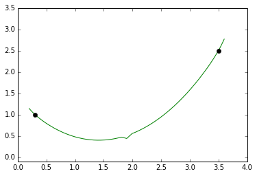
Further, even in leaf cells, the gradient of the distance is discontinuous between adjacent leaf cells. This lack of smoothness can cause nonphysical behavior in the solution. To see this, consider the same one-dimensional cable problem as above, but instead of using a smoothed, approximate distance function, we use an exact Euclidean distance. The gradient of Euclidean distance is discontinuous at the medial axis, and you can see the artifact propogated all the way to the solution.
Regardless of the bugs I find when I have time to fix the code, I think a stable simulation will require a distance smoothing routine for the essential boundary conditions. I don't think this will be terribly difficult -- I can imagine a two step procedure for this. The first step sweeps across the ASDF, filling in the missing distance values, while the second smooths over the cell bounaries.
The first test simulation took less than a minute on my laptop to evaluate all the integrals. This is actually very encouraging, because all of the allocation procedures were imlemented naively and can likely be sped up. After getting the system workign, I want to compared required time to a mesh-based FEA procedure.
Further, it will be very interesting to allocate the shape functions based on the ASDF refinements. The geometric detail isn't a perfect proxy for the field detail (e.g. the strain field detail), but considering that mesh based approaches tend to equate these two, it is a reasonable strategy to investigate.
Finally, this simulation should be vetted against both an analytically soluble case (e.g., tension in a cylinder) and a physical measurement (i.e. with an Instron).
Lots of it! Answer all the evaluation questions!
I wrote most of this project in C, in a branch of the kokopelli repository. Following Matt's great example, I used ctypes to expose the C functions to python, where I could script the generation of ASDFs, allocate shape functions over them, solve the linear systems, and display the results.
For class, here is some very-much-in-progress sample code:
Initial brainstorming of other ideas for my final project is documented here.