Final Project Discussion
what question(s) are you asking?
Is it possible to condense a large recurrent network into a cannonical set of nonlinear responses. I took to approaches to this. One was to use PCA to identify the similarity between neurons and then merge based on this criterion. Because I was not able to merge more than a dozen or so neurons in this way I then tried merging these neurons and iteratively training. The thinking behind this was that if I could merge several neurons and still "lie close" to a solution that training would take me towards the nearest solution. Next I asked how the types of solutions that a network can converge to depend on the size of the network.
what's the background and prior art?
I didn't find any work condensing trained RNNs to small cannonical sets. Presumably this is because the bulk of RNN work is done in areas where we want large networks with lots of expressive power. The goal of this project was to see if there is a relatively simple way to reduce RNNs to smaller networks where it is more tractable to study the dynamics of the network in detail.
what sources did you use?
I used a library private library for training the reccurent networks using conjugate gradient and hessian free methods that was developed by a post-doc in my lab as well as the behavioral analog developed in the lab for prior work.
what did you do?
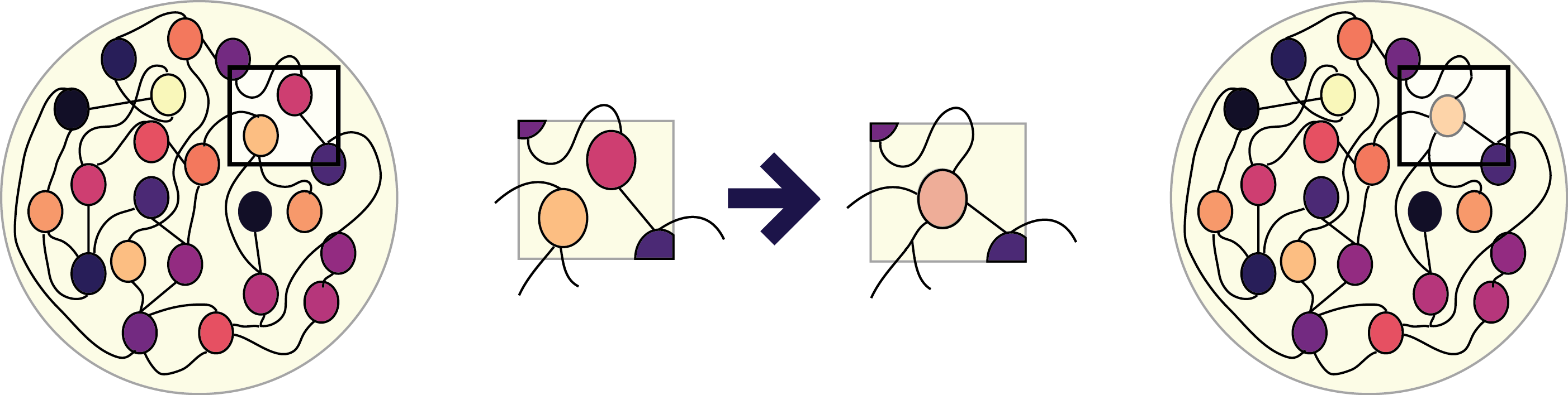
I used PCA to categorize neurons into different groups and then tried to merge neurons using differnent critera (this involves essentially passing weights from one neuron to another and deleting all of the weights from that neuron). Next I tried to perform this iteratively, training the network 100 times after each merging step and then
what worked, what didn't?
I wasnt able to condense more than a dozen or so neurons using PCA to choose, pairs. I also tried using correlation but obtained similar resuts. Next I tried to perform this process iteratively but I ended up with a ramping solution which is not similar to the network I started with. I looked a bit at how the size of the network affects not only the possible expressive power but also constrains the type of solutions the network can make
how did you evaluate progress?
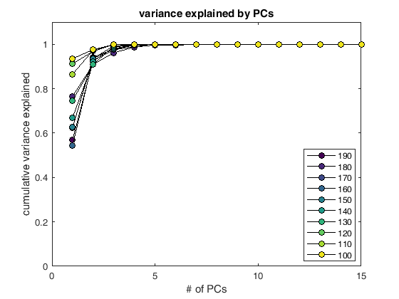
This was relatively easy because I wanted to obtain a network that could still do the task which I could assess simply by running network forward. I also looked at the PC's of the network and asked how many were required to
what are the implications for future work?
Perhaps there is something interesting related to the types of solutions found by RNNs that can be studied using a very simple task like this one.
SEMESTER PROJECT IDEAS:
The main thing that I want to get out of this project is to review some of the different ways that people use neural networks, not for machine learning but for modeling real neurons. To this end I started by doing several small projects making different "toy" networks getting an idea about how to do simple simulations of spiking neurons, small rate based recurrent networks, ring attractors etc. After doing this I turned to a larger reccurent network that was trained through hessian free back-propegation through time to preform an analog of a behavioral task that was developed and is used in a lab that I spend time in this past semester.
Initial Idea: Make a biophysical model of a syrinx and get it to produce vocalizations Simulate and oscillating membrane and manipulate the pressure in the organ to output different sound pressures that the ‘beak’
(https://en.wikipedia.org/wiki/Syrinx_(bird_anatomy)) The problem with this idea is that there seems to be a lot of work already done on this and I don’t see a clear way that I would like to build on what has already been done. For instance there is a lab in Argentina which basically works solely on my project idea (http://www.lsd.df.uba.ar/)
WEEK 1:
This week I wanted to get some intuition about about how to simulate spiking neurons so I undertook the relatively simple task of putting together a simulation of a single spiking neuron using a description of the differential equation that descibes the ionic currents
%matplotlib inline
import matplotlib.pyplot as plt
import numpy as np

########## PARAMETERS ########## (see Tesileanu et al.,)
n = 300 #number of neurons
Vrest = -72.3 #reset potential in mV
Vthr = -48.6 #threshold in mV
tMEM = 24.5 #membrane time constant in ms
ref = 10 #refractory period in ms
tAMP = 6.3 #ampa time constant in ms
tNMDA = 81.5 #nmda time constant in ms
tINH = 20 #inhibitory time constant in ms
R = 353 #MegaOhms input resistance
########## TEST CASE ########## (using random current and inhibitory input)
tstep = 5000
V = np.zeros(tstep)
V[0] = Vrest
I = (np.random.rand(tstep)-0.3)
inh = np.random.rand(tstep)*100
#inh = 35*np.ones(tstep)
j = 0

spike = False

for i in range (1,tstep):
    if V[i-1] > Vthr:
        spike = True


    if j == ref:
        spike = False

    if spike == True:
        spike = True
        if j < 1:
            V[i] = 50 + np.random.rand(1)*25
        else:
            V[i] = Vrest-20+j + np.random.rand(1)*25
        j+=1


    if spike == False:
        j = 0
        dV = (1/tMEM)*(Vrest - V[i-1] + R*(I[i-1]) - inh[i-1])
        V[i] = V[i-1]+dV

fig =plt.figure(figsize=(6, 3), dpi= 180, facecolor='w', edgecolor='k')
plt.plot(V[0:500],color = 'k', linewidth = 0.5)
plt.plot(np.ones(500)*Vthr,'--r', linewidth = 1)
plt.plot(np.ones(500)*Vrest,'--b', linewidth = 1)

fig =plt.figure(figsize=(6, 3), dpi= 180, facecolor='w', edgecolor='k')
plt.plot(V,color = 'k', linewidth = 0.5)
plt.plot(np.ones(tstep)*Vthr,'--r', linewidth = 1)
plt.plot(np.ones(tstep)*Vrest,'--b', linewidth = 1)


Other possible ways?
$$ \text{the differential equation governing the voltage of neuron i in this model is given by} \\ {V_i} = V_{i-1} + e^{\frac{R*(I_i^{AMPA}+I_i^{NMDA})}{\tau_m}} - V_{inh} $$$$ \tau_{m} \quad \text{is the time constant of the membrane}\\ $$$$ V_{r} \quad \text{is the resting potential of the neuron}\\ $$$$ I_i^x \quad \text{current input of type x into neuron i at time t}\\ $$$$ V_i \quad \text{is the voltage of neuron i at time t}\\ $$$$ R \quad \text{is the input resistance}\\ $$WEEK 2:
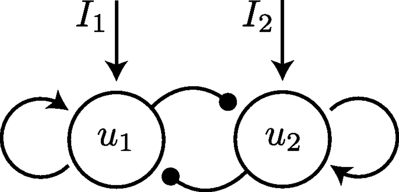
This week I put together a simple two neuron recurrent network as shown below and simply tested different inputs into this network. It has a diagonal weight matrix and thus input along the eigenvectors excite of the of the two modes of the network as shwon in the animation
display(HTML("<table><tr><td><img src='F2.large.jpg'></td><td><img src=''></td></tr></table>"))
 |
Gaining intuition for simple recurrence in small networks
%matplotlib inline
import matplotlib.pyplot as plt
import numpy as np
from IPython.display import HTML
from numpy import linalg as LA
import matplotlib.animation as animation

## SET PARAMETERS ##
tstep = 800
M = np.array([(0,0.8),(0.8,0)])
v = np.zeros([2,tstep])
h = np.zeros([2,tstep])
val,vec = LA.eig(M)
h[0,30:40] = np.ones([1,10])
h[1,130:140] = np.ones([1,10])
h[:,230:240] = np.ones([2,10])
h[0,330:340] = -np.ones([1,10])
h[1,430:440] = -np.ones([1,10])
h[:,530:540] = -np.ones([2,10])
h[:,630:640] = np.ones([2,10])
h[0,630:640] = h[0,630:640]*vec[0,1]
h[1,630:640] = h[1,630:640]*vec[1,1]
h[:,730:740] = np.random.rand(2,1)*np.ones([2,10])
tao = 4

## RUN DYNAMICS FORWARD ##
for i in range(1,tstep):
    dv = (1/tao)*(-v[:,i-1] + np.dot(M,v[:,i-1]) + h[:,i-1]);
    v[:,i] = v[:,i-1]+dv;
# First set up the figure, the axis, and the plot element we want to animate
fig = plt.figure(figsize=(5, 3), dpi= 180, facecolor='w', edgecolor='k')
#ax = plt.axes(xlim=(-3, 3), ylim=(-3, 3))
ax1 = fig.add_subplot(121, xlim=(-3,3), ylim=(-3,3))
ax2 = fig.add_subplot(122, xlim=(-3,3), ylim=(-3,3))

line, = ax1.plot([], [], lw=1, color = 'k',)
line2, = ax1.plot([], [], 'o',lw=1, color = 'k',markersize=5)

line3, = ax2.plot([], [], '-',lw=3, color = 'k')
ax1.grid()
ax2.grid()

# initialization function: plot the background of each frame
def init():
    line.set_data([], [])
    line2.set_data([], [])
    line3.set_data([], [])
    return line, line2, line3

# animation function.  This is called sequentially
def animate(i):
    x = v[0,1:i+1]
    y = v[1,1:i+1]
    line.set_data(x, y)
    line2.set_data(v[0,i+1], v[1,i+1])
    line3.set_data([0,h[0,i+1]], [0,h[1,i+1]])
    return line,

# call the animator.  blit=True means only re-draw the parts that have changed.
anim = animation.FuncAnimation(fig, animate, init_func=init,
                               frames=799, interval=20, blit=True)

ax1.plot([0,vec[0,0]],[0,vec[1,0]],'r-',linewidth = 0.5)
ax1.plot([0,vec[0,1]],[0,vec[1,1]],'r-',linewidth = 0.5,label='eigenvectors')

handles, labels = ax1.get_legend_handles_labels()
ax1.legend(handles, labels)

ax1.set_title("network activity")
ax2.set_title("network input")
plt.tight_layout()
plt.close()
HTML(anim.to_html5_video())
WEEK 3:
Reproduce respiratory model from Rubin et al., 2009
#%%
import matplotlib.pyplot as plt
import numpy as np
from numpy import linalg as LA
#%% parameters

# Conductances:
C=20
g_Nap=0
g_k=5.0
g_AD=10.0
g_L=2.8
g_synE=10.0
g_synI=60

# Reversal potentials:
E_Na=50
E_k=-85
E_L=-60
E_synE=0
E_synI=-75

# weights
a_12=0.4
b = np.array([(0,0,0.3,0.2),(0,0,0.05,0.35),(0,0.25,0,0.1),(0,0.35,0.35,0)])
c = np.array([(0.115,0.07,0.025),(0.3,0.3,0),(0.63,0,0),(0.33,0.4,0)])

V_half=-30
kV = np.array([8,4,4,4]) #output slopes
tau_naMax=6e3
tau_AD = np.array([np.nan,2e3,1e3,2e3]) # adaptation time constants
k_AD = np.array([np.nan,0.9,0.9,1.3]) # adaptation paramters
d = np.ones(3) #external inputs

#%%
# lambda functions
f = lambda x, y: 1/(1+np.exp(-(x-V1_2)/y))
hInfNaP= lambda u: 1./(1+np.exp((u+48)/6))
mNaP= lambda u: 1./(1+np.exp(-(u+40)/6))
TauhNaP= lambda u,tauMax: tauMax/np.cosh((u+48)/12)
mK= lambda u: 1./(1+np.exp(-(u+29)/4))
f= lambda u, kv: 1./(1+np.exp(-(u-V_half)/kv))

#%%
# Initialize variabiles
numsteps=100000
dt=1e-1
h_NaP=np.zeros(numsteps)
I_K=np.zeros(numsteps)
I_NaP=np.zeros(numsteps)
V = np.zeros((4,numsteps))
V[:,0] = np.array([-50.82041612, -36.22710468, -36.83931196, -41.83978807])
I_AD = np.zeros((4,numsteps))
m_AD = np.zeros((4,numsteps))
I_L = np.zeros((4,numsteps))
I_synE = np.zeros((4,numsteps))
I_synI = np.zeros((4,numsteps))

#%%
for j in range(0,numsteps-1): #TIME LOOP
    # updating parameters
    tau_hNaP=TauhNaP(V[0,j],tau_naMax)
    h_NaP[j+1]=dt*1/tau_hNaP*(-h_NaP[j]+hInfNaP(V[0,j])+h_NaP[j])
    I_K[j+1]=g_k*(mK(V[0,j])**4)*(V[0,j]-E_k)
    I_NaP[j+1]=g_Nap*mNaP(V[0,j])*h_NaP[j+1]*(V[0,j]-E_Na)
    # get inputs
    inhibitory_activation = np.dot(b,f(V[:,j],kV))
    excitatory_activation = np.dot(c,d)

    for i in range(0,4): # NEURON LOOP
        m_AD[i,j+1]=dt*1/tau_AD[i]*(-m_AD[i,j]+k_AD[i]*f(V[i,j],kV[i]))+m_AD[i,j]
        I_AD[i,j]=g_AD*m_AD[i,j+1]*(V[1,j]-E_k)
        I_L[i,j]=g_L*(V[i,j]-E_L)
        if i == 1:
            I_synE[i,j]=g_synE*(V[i,j]-E_synE)*(a_12*f(V[0,j],kV[0])+excitatory_activation[i])
        else:
            I_synE[i,j]=g_synE*(V[i,j]-E_synE)*excitatory_activation[i]
        I_synI[i,j]=g_synI*(V[i,j]-E_synI)*inhibitory_activation[i]
        if i == 0:
            V[i,j+1]=dt*1/C*(-I_NaP[j]-I_K[j]-I_L[i,j]-I_synE[i,j]-I_synI[i,j])+V[i,j]
        else:
            V[i,j+1]=dt*1/C*(-I_AD[i,j]-I_L[i,j]-I_synE[i,j]-I_synI[i,j])+V[i,j]
fig = plt.figure(figsize=(4, 5), dpi= 180, facecolor='w', edgecolor='k')

plt.subplot(4, 1, 1)
plt.plot(np.arange(0,numsteps)*dt/600,f(V[0,:],kV[0]),'k',linewidth = 2)
plt.title('neuron 1')
plt.subplot(4, 1, 2)
plt.plot(np.arange(0,numsteps)*dt/600,f(V[1,:],kV[1]),'r',linewidth = 2)
plt.title('neuron 2')
plt.subplot(4, 1, 3)
plt.plot(np.arange(0,numsteps)*dt/600,f(V[2,:],kV[2]),'b',linewidth = 2)
plt.title('neuron 3')
plt.subplot(4, 1, 4)
plt.plot(np.arange(0,numsteps)*dt/600,f(V[3,:],kV[3]),'orange',linewidth = 2)
plt.title('neuron 4')
plt.tight_layout(h_pad=0)
plt.show()

fig = plt.figure(figsize=(4, 2), dpi= 180, facecolor='w', edgecolor='k')
plt.plot(np.arange(0,numsteps)*dt/600,f(V[0,:],kV[0]),'k',linewidth = 1)
plt.plot(np.arange(0,numsteps)*dt/600,f(V[1,:],kV[1]),'r',linewidth = 1)
plt.plot(np.arange(0,numsteps)*dt/600,f(V[2,:],kV[2]),'b',linewidth = 1)
plt.plot(np.arange(0,numsteps)*dt/600,f(V[3,:],kV[3]),'orange',linewidth = 1)
plt.title('respiratory oscillator')
plt.show()


WEEK 4:
Make a ring attactor network and get it to move
display(HTML("<table><tr><td><img src='x587.png'></td><td><img src=''></td></tr></table>"))
 |
import numpy as np
import matplotlib.pyplot as plt
N = 100
h0 = 2
h1 = 1
T = 2
tao = 1
step = 0.01
numsteps = 1000
w1 = 1
w0 = 0.9

def rect(x):
    x[x <= 0] = 0;
    a = x;
    return(a)


a0 = np.random.rand(N,1)
ptheta = np.ones((N,1))*np.arange(N).reshape((N, 1))
ptheta *= ((2*np.pi)/(N-1))
W = np.zeros((N,N))
for i in range(0,N-1):
    for j in range(0,N-1):
        W[i,j] = (1/N)*(w0+w1*np.cos(ptheta[i]-ptheta[j]))

a = a0;
ahist = np.zeros((N,numsteps))
for ii in range(0,numsteps):
    da = -a + rect(np.dot(W,a)+h0+(h1*np.cos(np.roll(ptheta,ii)))-T)
    a += da*step
    ahist[:,ii] = a.T
fig = plt.figure(figsize=(6, 6), dpi= 180, facecolor='w', edgecolor='k')
plt.imshow(ahist,cmap = 'RdBu')

# First set up the figure, the axis, and the plot element we want to animate
fig = plt.figure(figsize=(5, 3), dpi= 180, facecolor='w', edgecolor='k')
ax = plt.axes(xlim=(0, 100),ylim=(0, 1.5))

line, = ax.plot([], [], lw=2, color = 'k',marker = 'o')
ax.grid()

# initialization function: plot the background of each frame
def init():
    line.set_data([], [])
    line2.set_data([], [])
    line3.set_data([], [])
    return line, line2, line3

# animation function.  This is called sequentially
def animate(i):
    x = np.arange(0.,100.)
    y = ahist[:,i]
    line.set_data(x, y)
    #line2.set_data(v[0,i+1], v[1,i+1])
    #line3.set_data([0,h[0,i+1]], [0,h[1,i+1]])
    return line,

# call the animator.  blit=True means only re-draw the parts that have changed.
anim = animation.FuncAnimation(fig, animate, init_func=init,
                               frames=1000, interval=15, blit=True)


ax.set_title("moving ring attractor bump")

plt.tight_layout()
plt.close()
HTML(anim.to_html5_video())
Introduction to the task etc.
Recently there have been several studies in systems neuroscience which have demonstrated that you can get RNN's to exhibit many features of neural data from animals performing behavioral tasks but training networks to perform analog tasks.
(see: http://www.nature.com/nature/journal/v503/n7474/full/nature12742.html
http://www.nature.com/neuro/journal/v18/n7/abs/nn.4042.html)
The observation that many of the individual units, the principal componenents and the average activity can look so similart to neural data has suggested to many that this is can be a useful model of neural activity during behavior despite the fact that these networks are trained with contemporary techniques which are extremely implausable biologically. For my project I asked if I could take a network trained in such as task and reduce it to a set of cannonical units. This makes sense for several reasons: First although 200-500 unit RNNS are relatively simple from a machine learning point of view it would be useful to have a smaller version of the network which captured the primary features of the activity. PCA of the activity can accomplish this in a way but doesn't allow the description of the input output relationships or hypotheses about functional relationships between units.
Cue_Set_Go Task http://www.nature.com/neuro/journal/v13/n8/full/nn.2590.html
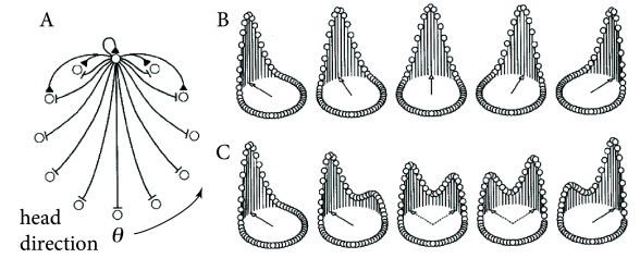
I used a network trained in a timing task which is an analog of a task monkeys have been trained to perform. During recordings in one frontal cortical area it was observed that there are many neurons which display nonlinearities which are invaraint to the timing condition but which stretch to fill the necessary time. Training a RNN in the analog shown below results in large set of nonlinear activity profiles which stretch in time.
The training itself was done using James Maarten's conjugate gradient code (Deep Learning via Hessian-free Optimization) which can befound on his website with his demo code http://www.cs.toronto.edu/~jmartens/research.html
Two important papers from which the code comes from
http://www.cs.toronto.edu/~jmartens/docs/Deep_HessianFree.pdf
http://www.cs.toronto.edu/~jmartens/docs/RNN_HF.pdf
There is a nice and thourough chapter here http://www.cs.utoronto.ca/~jmartens/docs/HF_book_chapter.pdf
(This was done in MATLAB... and I don't have the MATLAB kernel working so there is no code in the notebook at the moment)
Characterizing my network
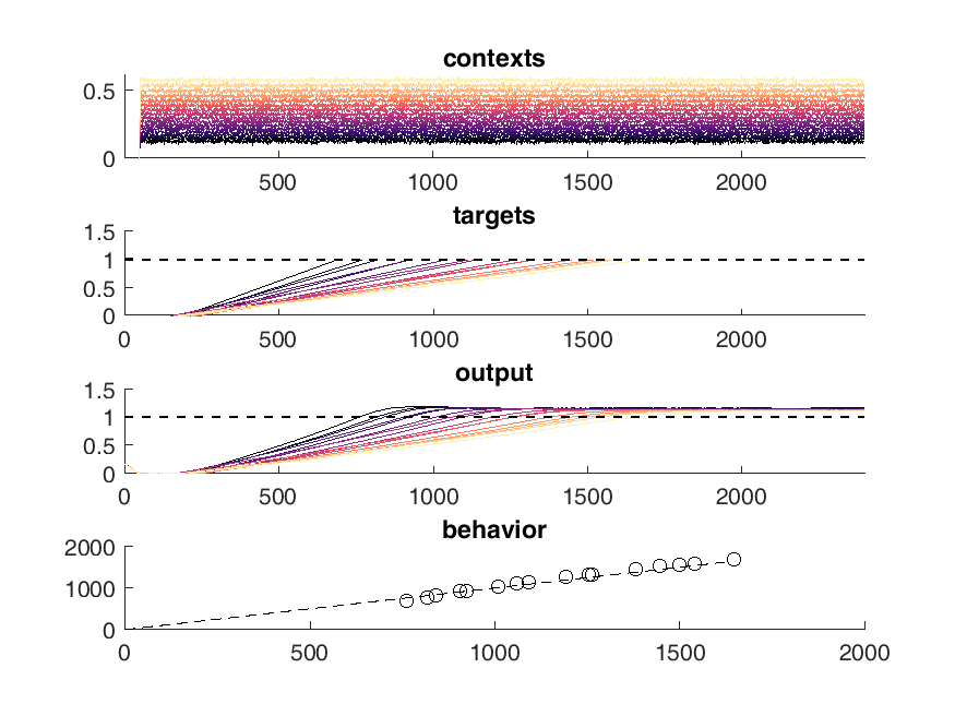
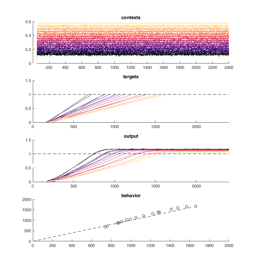
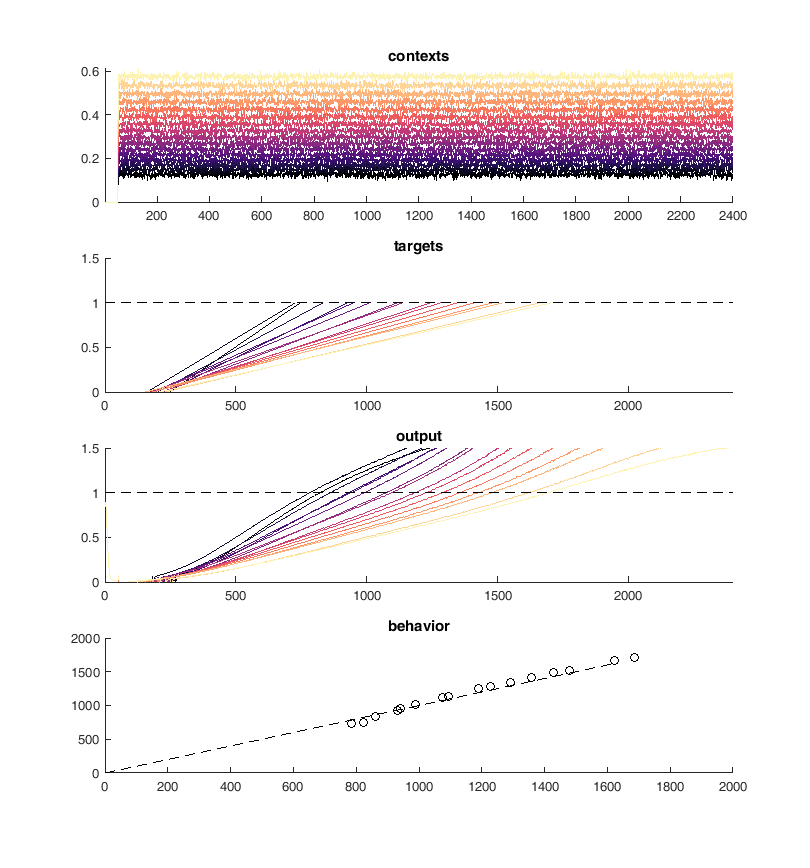
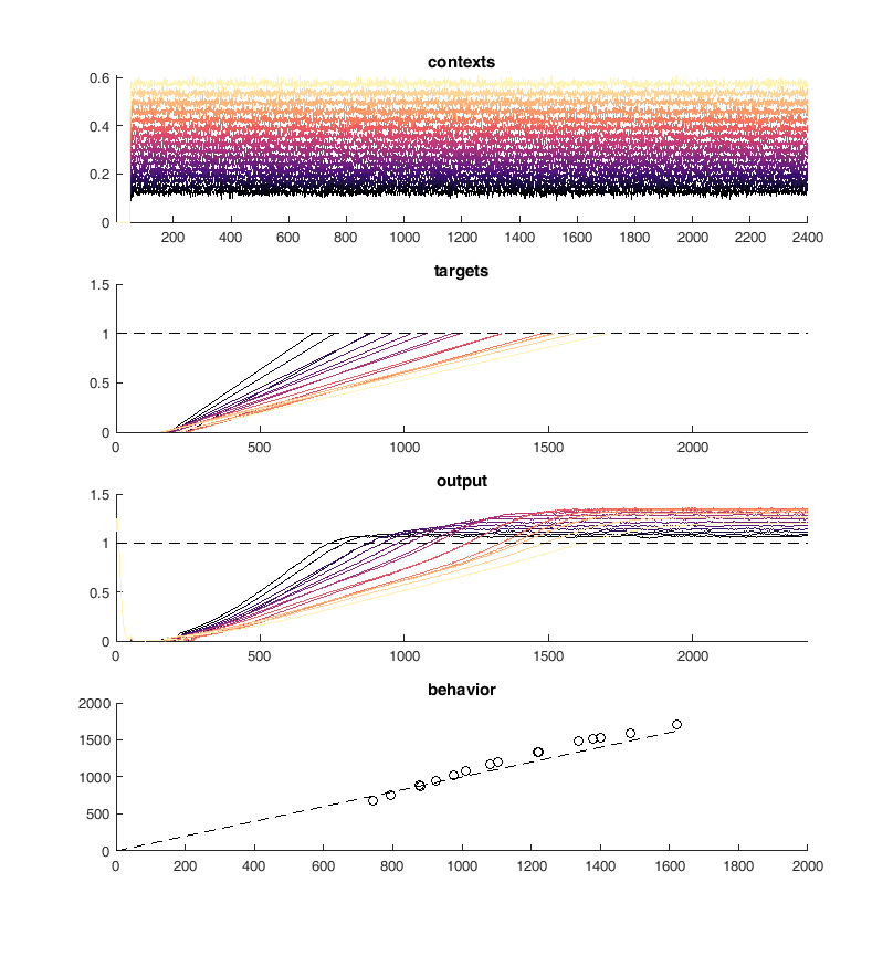
Here is an example of the output of the network. On the top panel you can see the inputs to the network which are constant steps. Each of these inputs is matched with a particular output slope of the ramp which is meant to represent the timing. The network should produce a steady ramp and the produced timing of the network is when the ramp reaches a value of one. A second input to the network tells the network when to begin ramping so it must wait for this cue.
The target behavior is given in the second panel and the actual network behavior is shown at the bottom. This output is the activity of one unit. Neurons are connected all to all.
display(HTML("<table><tr><td><img src='original network behavior.png'></td><td><img src=''></td></tr></table>"))
 |
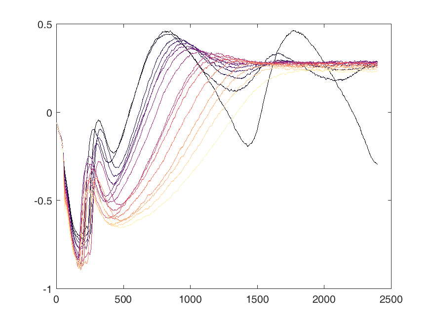
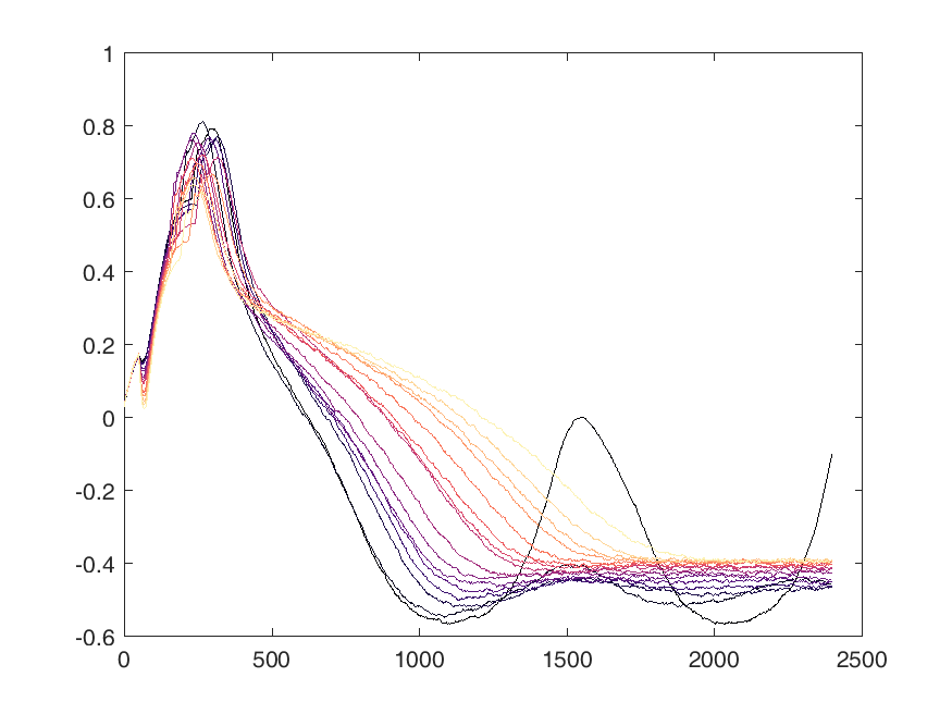
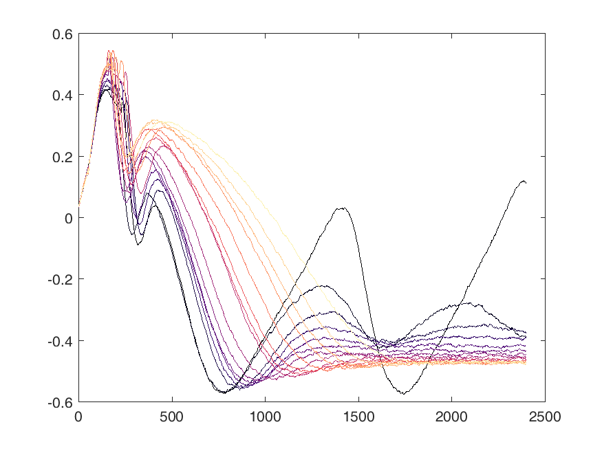
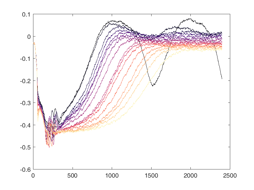
Shown below are examples of what the activity of the reccurent units look like during the task colored by context. The main point is that neurons do not simple ramp as you might expect but rather more complex.
from IPython.display import HTML, display
display(HTML("<table><tr><td><img src='unit 52 of 16.png'></td><td><img src='unit 58 of 16.png'></td></tr></table>"))
display(HTML("<table><tr><td><img src='unit 56 of 16.png'></td><td><img src='unit 59 of 16.png'></td></tr></table>"))
 |  |
 |  |
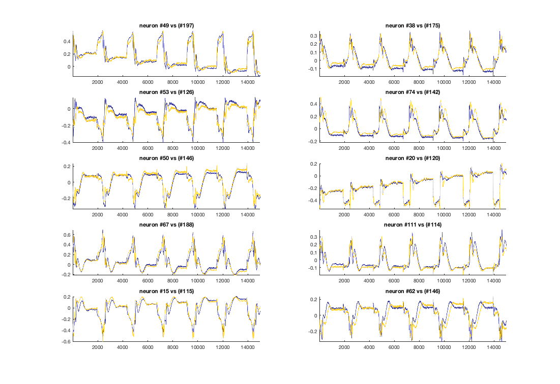
Identifying neurons using PCA
display(HTML("<table><tr><td><img src='neuron_20_3.7.16.png'></td><td><img src=''></td></tr></table>"))
 |
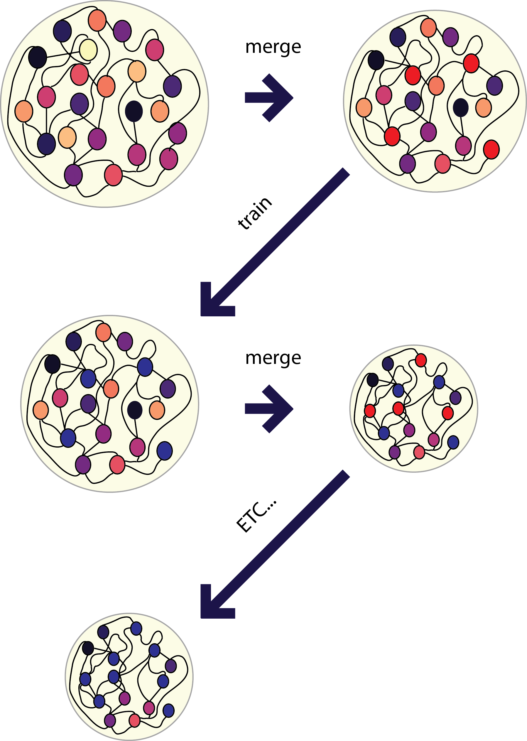
Take one process
display(HTML("<table><tr><td><img src='process.png'></td><td><img src=''></td></tr></table>"))
 |
from IPython.display import HTML, display
display(HTML("<table><tr><td><img src='5 merged network behavior.png'></td><td><img src='10 merged network behavior.png'></td></tr></table>"))
display(HTML("<table><tr><td><img src='16 merged network behavior.png'></td><td><img src='17 merged network behavior.png'></td></tr></table>"))
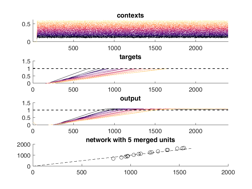 | 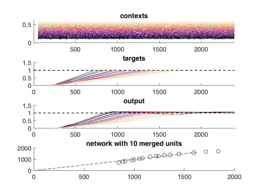 |
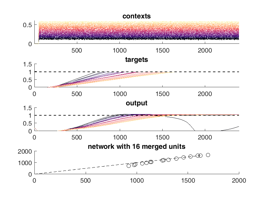 | 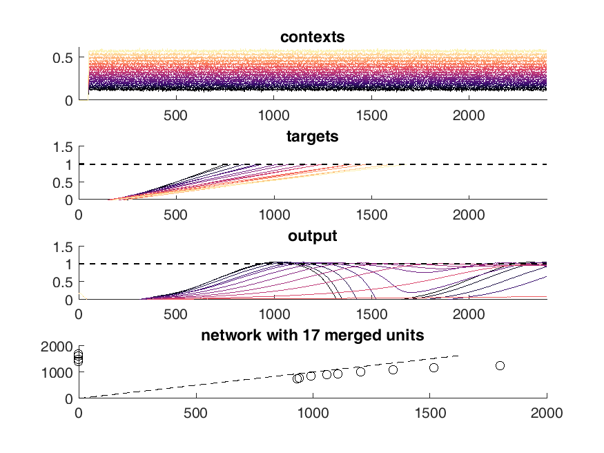 |
<img src="eigenvalue_spectrum.png",width=600,height=600>
Attempting to iteratively train the network
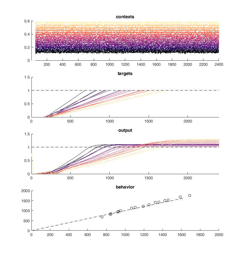
Next I tried to perform the above task iteratively. I used PCA to identify neurons with similar activity and non-linear relationships to the "contexts". First I merged the 10 most similar pairs of neurons and then I trained 100 epochs of 100 iterations of conjugate gradient descent each. Performing this method I was able to continuously reduce the size of the network while maintaining performance on the "behavioral task".
display(HTML("<table><tr><td><img src='pcatrainB.png'></td><td><img src=''></td></tr></table>"))
 |
190 - 180
display(HTML("<table><tr><td><img src='merge10trained.png'></td><td><img src='merge20trained.png'></td></tr></table>"))
 |  |
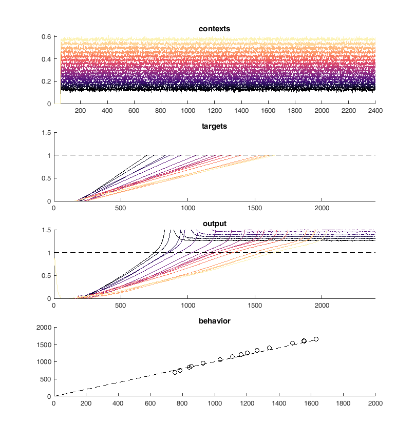
170 - 160
display(HTML("<table><tr><td><img src='merge40trained.png'></td><td><img src='merge40trained.png'></td></tr></table>"))
 | |
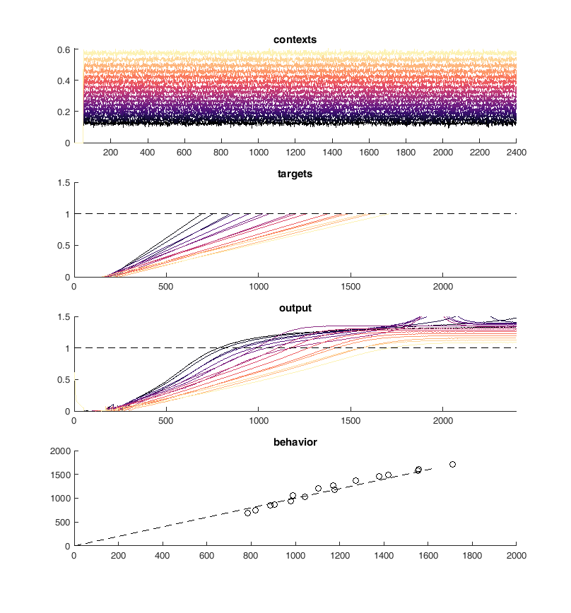
150 - 140
display(HTML("<table><tr><td><img src='merge50trained.png'></td><td><img src='merge60trained.png'></td></tr></table>"))
 |  |
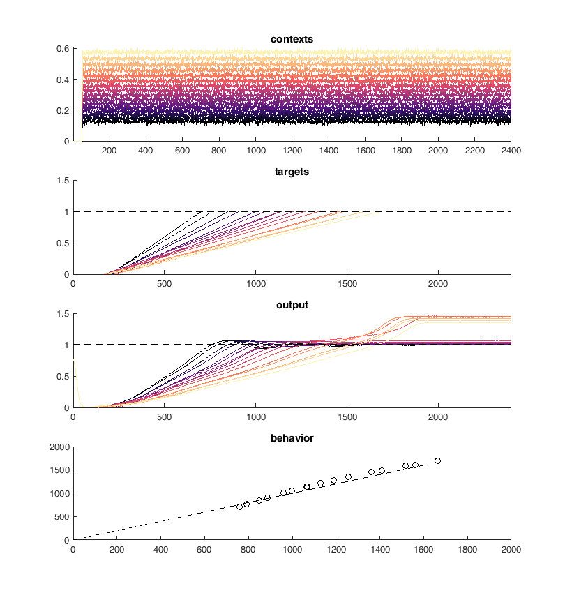
130 - 120
display(HTML("<table><tr><td><img src='merge70trained.png'></td><td><img src='merge80trained.png'></td></tr></table>"))
 |  |
110 - 100
display(HTML("<table><tr><td><img src='merge90trained.png'></td><td><img src='merge100trained.png'></td></tr></table>"))
 |  |
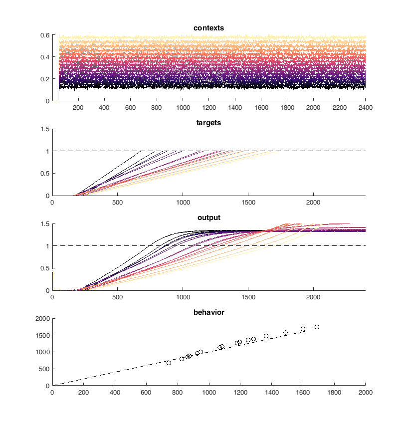
Discussion of resultant network
This worked well but I was unable to retain the type of solution in the original network which was the whole point of this process. I ended up with a simple set of ramps up and down aka an integrator
display(HTML("<table><tr><td><img src='allPCsC.png'></td><td><img src='1stPCs.png'></td></tr></table>"))
 |  |
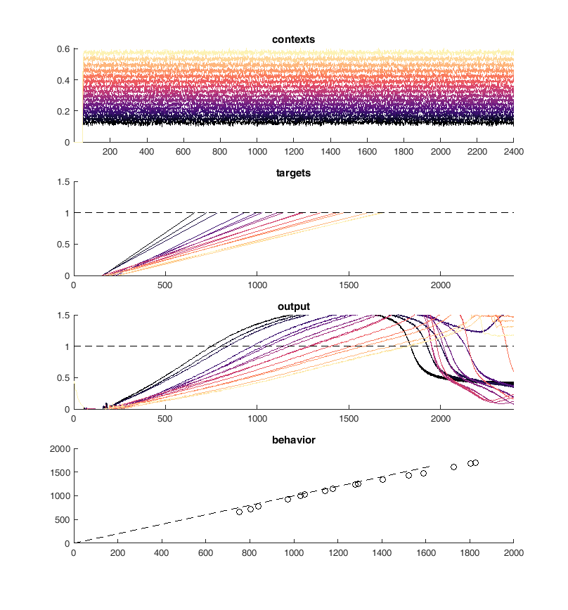
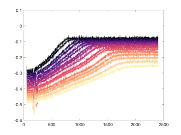
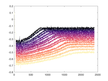
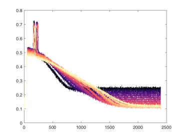
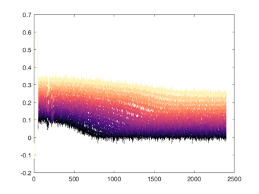
Units are ramping - Network finds a different solution
display(HTML("<table><tr><td><img src='Picture3.png'></td><td><img src='Picture4.png'></td></tr></table>"))
display(HTML("<table><tr><td><img src='Picture5.png'></td><td><img src='Picture6.png'></td></tr></table>"))
 |  |
 |  |
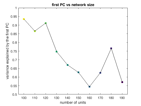
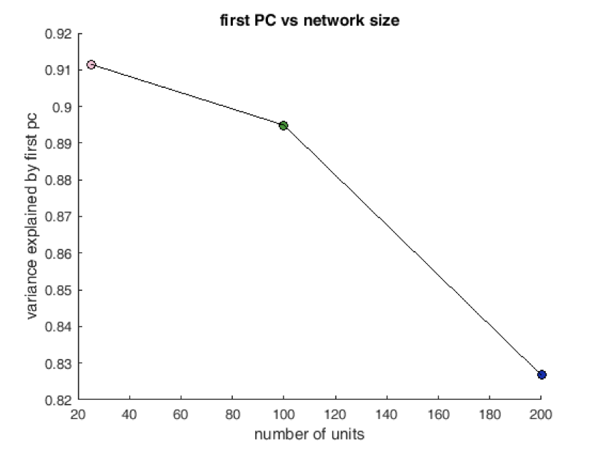
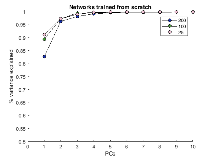
Preliminary (Perhaps this is general?)
Trained a set of different networks with various sizes from scratch ans asked how rich solutions were. Possible transition in solution type?
display(HTML("<table><tr><td><img src='Picture1.png'></td><td><img src='Picture2.png'></td></tr></table>"))
 |  |