The Nature of Mathematical Modelling

6.1

(a) Work out the first three cumulants C1, C2, and C3.

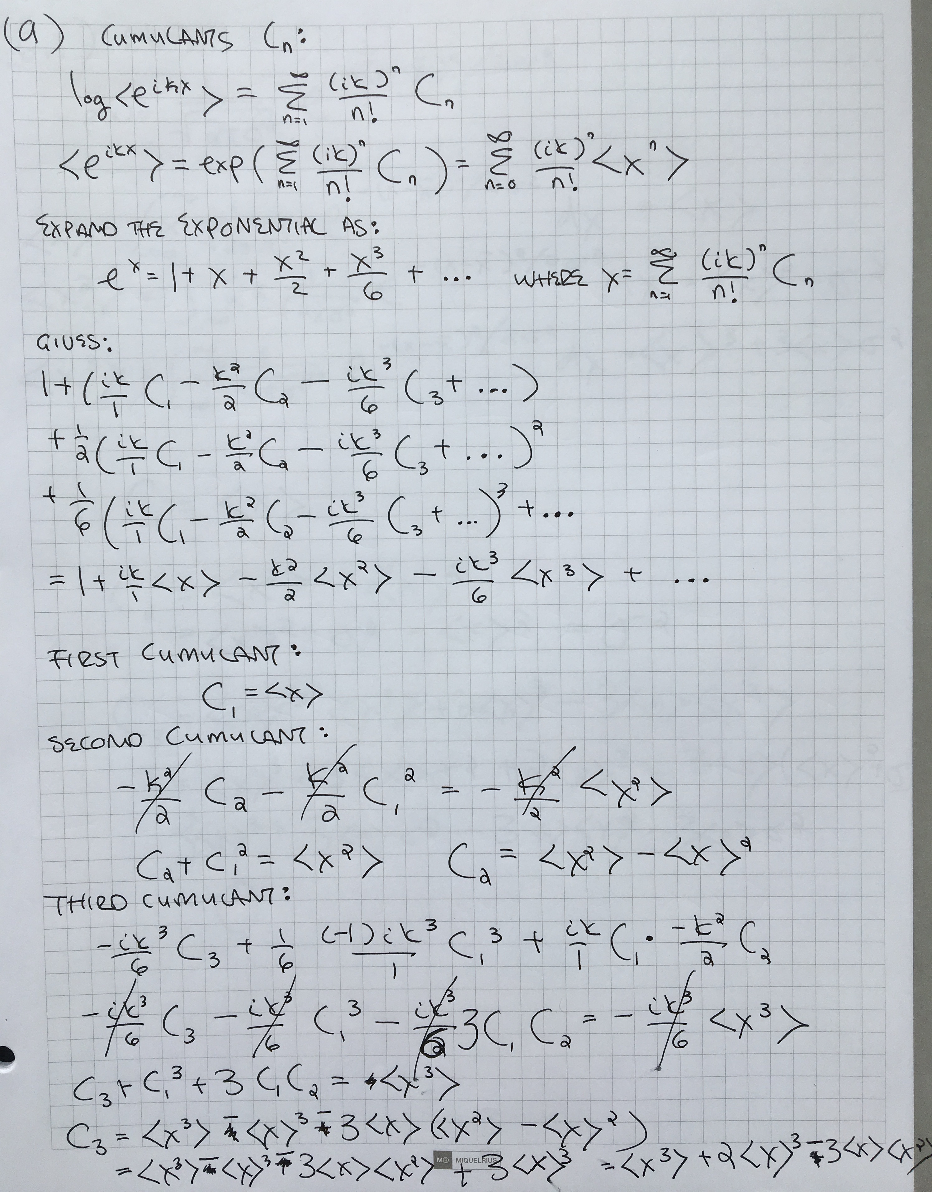
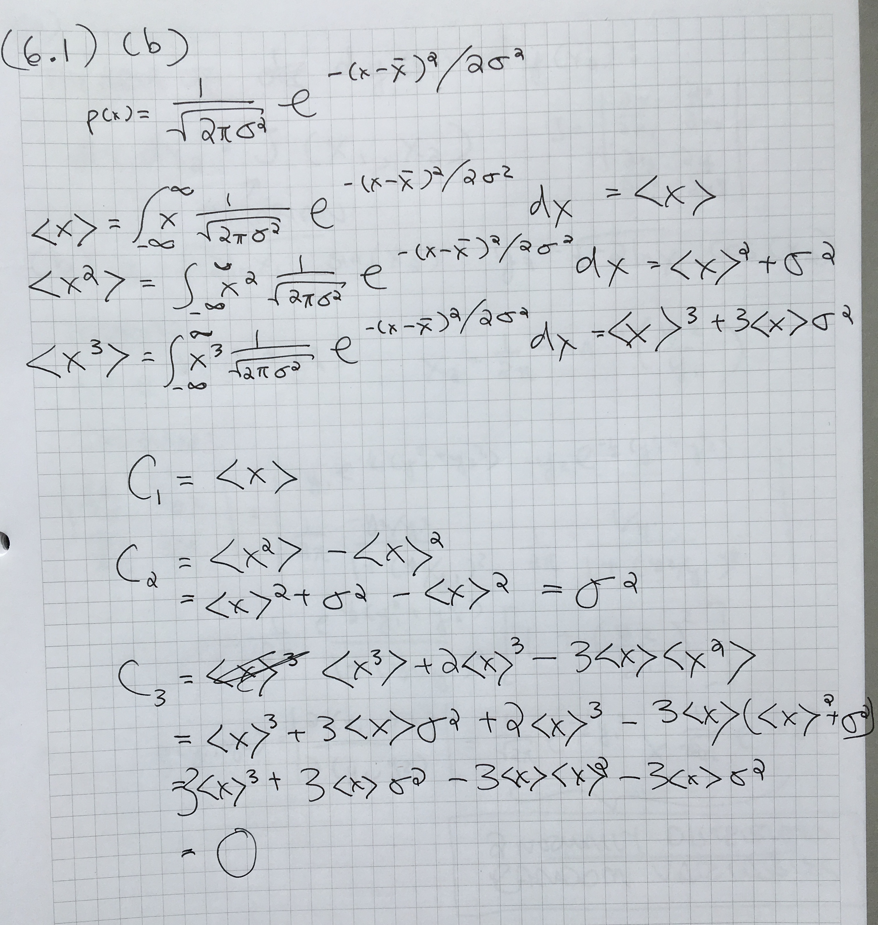
(b) Evaluate the first three cumulants for a Gaussian distribution

6.2

(a) If ~y(~x) = (y1(x1, x2), y2(x1, x2)) is a coordinate transformation, what is the area of a differential element dx1 dx2 after it is mapped into the ~y plane? Recall that the area of a parallelogram is equal to the length of its base times its height.

(b) Let y1 = p −2 ln x1 sin(x2) y2 = p −2 ln x1 cos(x2) . (6.78) If p(x1, x2) is uniform, what is p(y1, y2)?

(c) Write a uniform random number generator, and transform it by equation (6.78). Numerically evaluate the first three cumulants of its output.

              function createRandomNumberGenerator() {
                var a = 8121
                var b = 28411
                var c = 134456

                var previous = 1
                return function() {
                  previous = (b * previous + c) % a
                  return previous / a
                }
              }

              var randomNumberGenerator = createRandomNumberGenerator()

              function normallyDistributedNumberGenerator() {
                let u = 1 - randomNumberGenerator(), v = 1 - randomNumberGenerator()
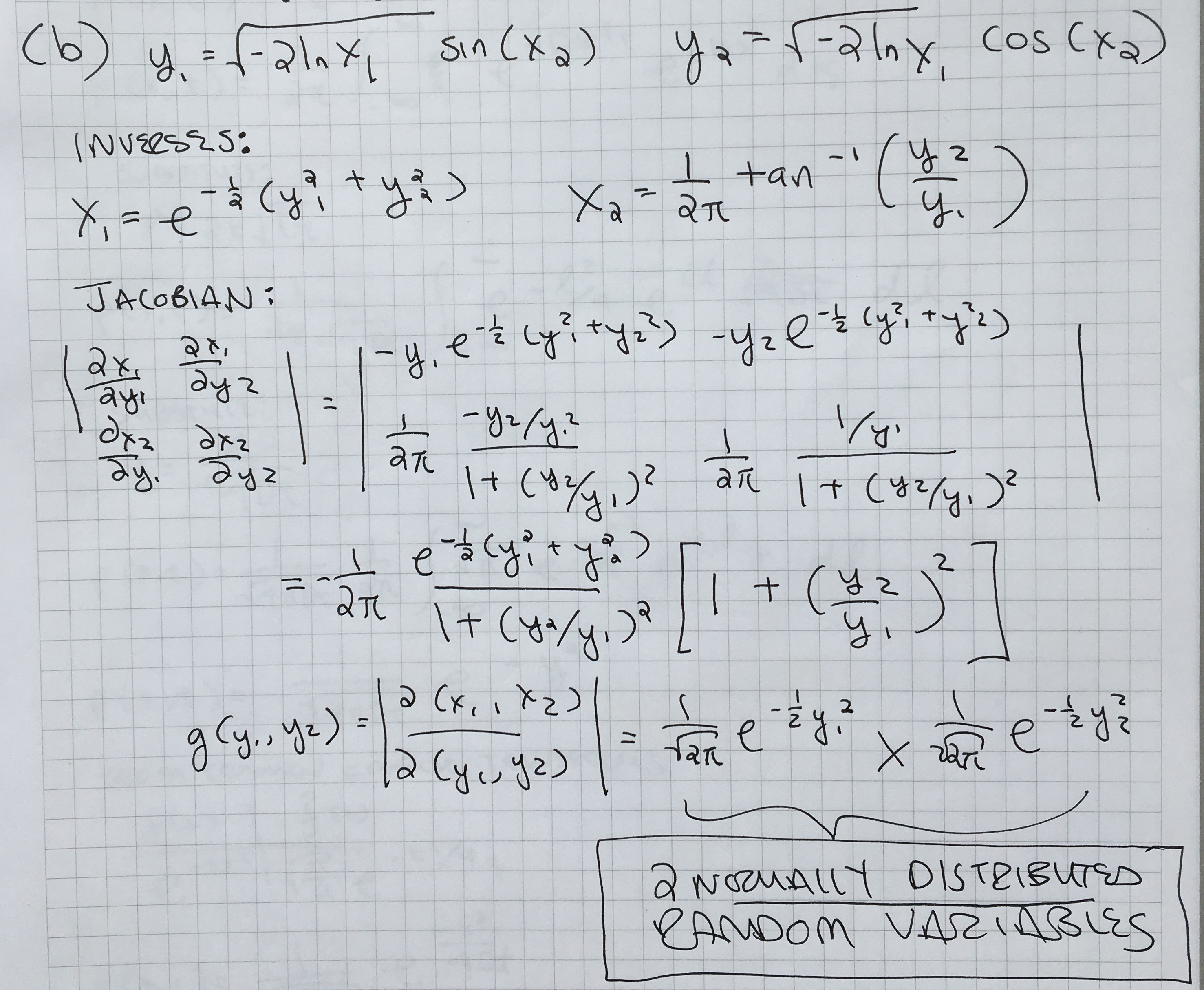
                return Math.sqrt(-2 * Math.log(u)) * Math.cos(2 * Math.PI * v) // this gives just the x-coordinates of the distribution
              }
            

6.4

(a) Use a Fourier transform to solve the diffusion equation (6.57) (assume that the initial condition is a normalized delta function at the origin).

(b) What is the variance as a function of time?

(c) How is the diffusion coefficient for Brownian motion related to the viscosity of a fluid?

(d) Write a program (including the random number generator) to plot the position as a function of time of a random walker in 1D that at each time step has an equal probability of making a step of ± 1. Plot an ensemble of 10 trajectories, each 1000 points long, and overlay error bars of width 3σ(t) on the plot.