The Nature of Mathematical Modelling

12.1

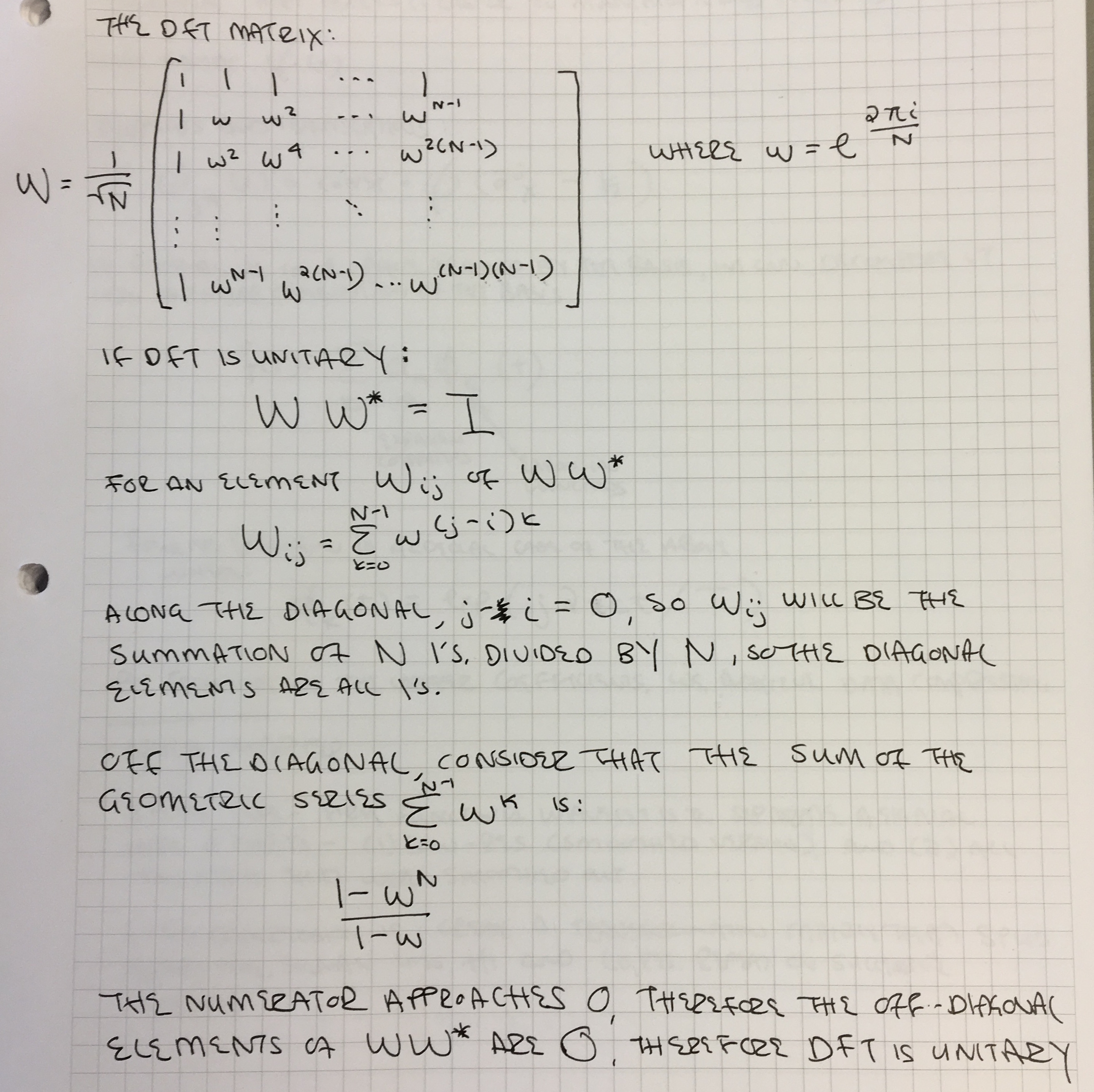
Prove that the DFT is unitary.

12.3

Consider a measurement of a three-component vector ~x, with x1 and x2 being drawn independently from a Gaussian distribution with zero mean and unit variance, and x3 = x1 + x2.

(a) Analytically calculate the covariance matrix of ~x

            x1^2         x1*x2       x1(x1 + x2)
            x2*x1        x2^2        x2(x1 + x2)
            x1(x1 + x2)  (x1 + x2)x2 (x1 + x2)^2

(b) What are the eigenvalues?

            0 0 0
            0 0 0
            0 0 0

(c) Numerically verify these results by drawing a data set from the distribution and computing the covariance matrix and eigenvalues.

(d) Numerically find the eigenvectors of the covariance matrix, and use them to construct a transformation to a new set of variables ~y that have a diagonal covariance matrix with no zero eigenvalues. Verify this on the data set.

12.4

Generate pairs of uniform random variables {s1, s2} with each component contained in [0, 1].

(a) Plot these data.

(b) Mix them (~x = A · ~s) with a square matrix A = [ 1 2; 3 1 ] and plot.

(c) Make ~x zero mean, diagonalize with unit variance, and plot.