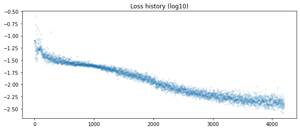
During the course of my PhD research, I have been been modeling and simulating a lot of dynamical systems (ODEs, PDEs, LBM, CA, neural networks,shape growth...). So I decided to take a closer look at the dynamical systems to see the best way to optimize these dynamical systems, given priors, which could consist of data (observations), or model guesses (constraints).
From my literature review I divided the dynamical systems optimization approaches into three categories:
I will go into detail about each category, what are the methods that can be used, small examples/implementations of these methods. I will at the end try to use all these methods for a particular case study: morphogenetic growth.
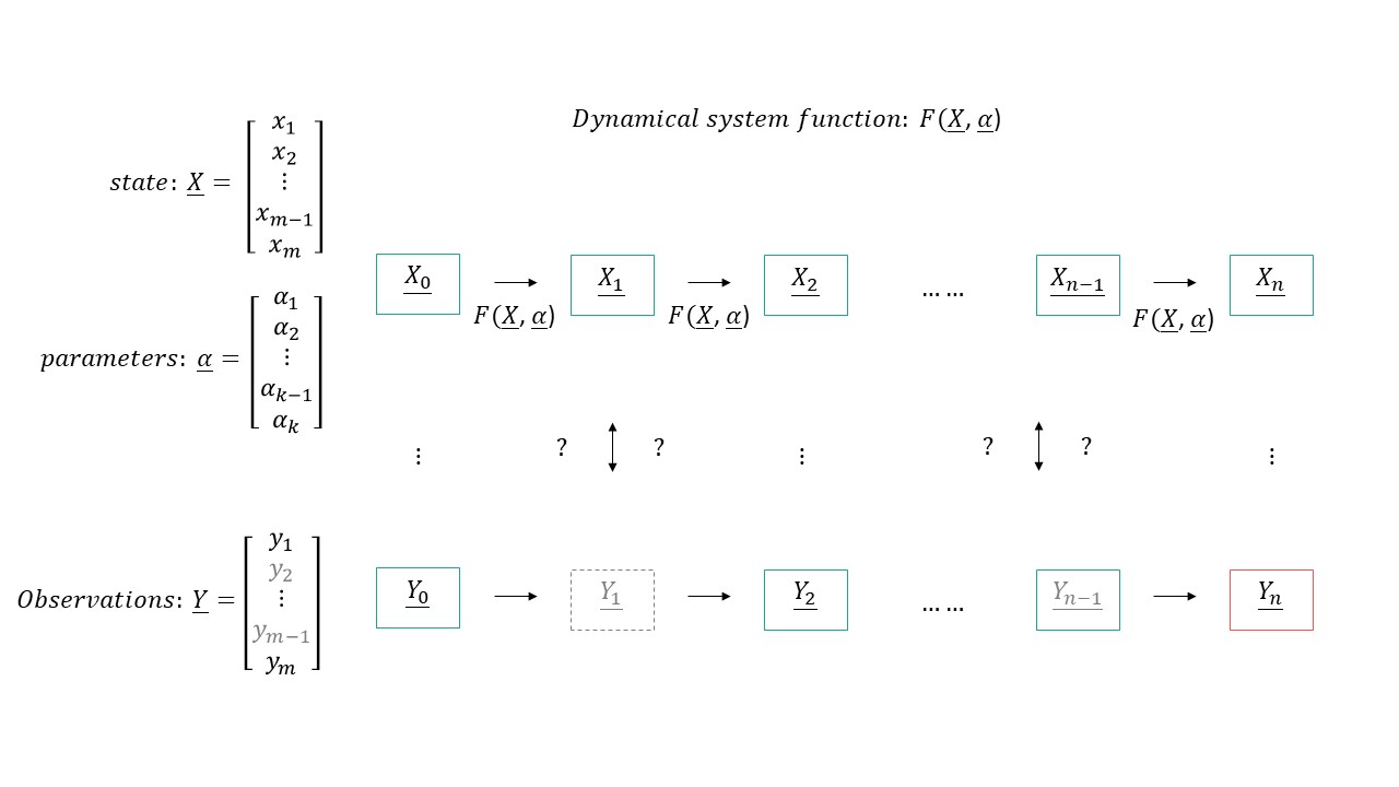
In the parameter estimation question, we usually know the start state $X_0$, we have a pretty good idea about the model (update function $F(X,\alpha)$) and given one or a series of observations $Y$, we want to find the best parameters $\alpha$ that would give the closes result to the observation $Y$.
The easiest way to approach the problem is to treat the dynamical system as a blackbox and use any of the non differentiable search methods we learned about in Week 8 (Nelder mead, CMAES, kernel density..). This however would take more time that is needed as you are not making use of any of the priors you have (your model, multiple observations..)
The first thing that comes to mind is to train the dynamical systems as if they are neural networks, in particular a recurrent neural network where the non linearity is the $F(X,\alpha)$ and we are looking for the weights (in our case $\alpha$).
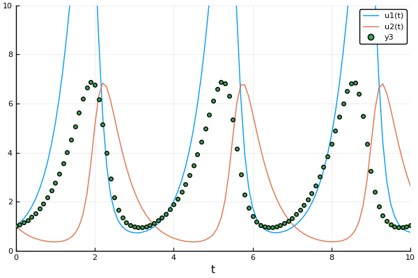
Example: Rabits vs wolves: Lotka volterra:
A detailed explanation about forward mode automatic differentiation could be found here and here
For an arbitrary nonlinear function $f$ with scalar output, we can compute derivatives by putting a dual number in. For example, with
$$d = d_0 + v_1 \epsilon_1 + \ldots + v_m \epsilon_m$$
we have that
$$f(d) = f(d_0) + f'(d_0)v_1 \epsilon_1 + \ldots + f'(d_0)v_m \epsilon_m$$
where $f'(d_0)v_i$ is the direction derivative in the direction of $v_i$. To compute the gradient with respond to the input, we thus need to make $v_i = e_i$.
However, in this case we now do not want to compute the derivative with respect to the input! Instead, now we have $f(x;\alpha)$ and want to compute the derivatives with respect to $\alpha$. This simply means that we want to take derivatives in the directions of the parameters. To do this, let:
$$x = x_0 + 0 \epsilon_1 + \ldots + 0 \epsilon_k$$ $$P = p + e_1 \epsilon_1 + \ldots + e_k \epsilon_k$$
where there are $k$ parameters. We then have that
$$f(x;\alpha) = f(x;\alpha) + \frac{df}{d\alpha_1} \epsilon_1 + \ldots + \frac{df}{dp_k} \epsilon_k$$
as the output, and thus a $k+1$-dimensional number computes the gradient of the function with respect to $k$ parameters.
Make use of the recursion using the chain rule on a computation graph. Recall that for $f(x(t),y(t))$ that we have: $$\frac{df}{dt} = \frac{df}{dx}\frac{dx}{dt} + \frac{df}{dy}\frac{dy}{dt}$$
given an evaluation of $f$, we can directly calculate $\frac{df}{dx}$ and $\frac{df}{dy}$. But now, to calculate $\frac{dx}{dt}$ and $\frac{dy}{dt}$, we do the next step of the chain rule:
$$\frac{dx}{dt} = \frac{dx}{dv}\frac{dv}{dt} + \frac{dx}{dw}\frac{dw}{dt}$$
What if we don't want to calculate the gradient because of the vanishing gradients effect, but we still want to make use the priors we have?
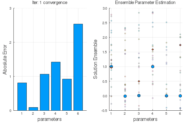
Ensemble methods are answer.
Steps:
Statistical Empirical Adjoint: $$ \delta E_1=E_1 E_2^T[E_2 E_2^T+R]^{-1}\delta E_2 $$
$E_1 \leftarrow E_2$ using $F(x,\alpha)$ the go back with the adjoint
Example: Mass Spring + Damper System:
Here we are trying to find $X_0$ given observations and a model (that could be incorrect).
Objective Function: $$J= \sum_{n=1}^{N} \frac{1}{2} [y_n-x_n]^2+ \lambda_n^T [x_n-F(x_{n-1}:\alpha)]$$
$$ \lambda_n=\Delta F |{x_n} \lambda{n+1} +(y_n-x_n) $$
1- Pendulum Properties:
$$ \dot{x}=A x $$ $$ x(0)= x_0 $$ $$ x(\delta t)= e^{A \delta t} x(0)$$
$$p_1=(m_1+m_2)L_1^2$$ $$p_2= m_2 L_2^2$$ $$p_3=m_2^2 L_1$$ $$p_4=(m_1+m_2) L_1$$ $$p_5=m_2 L_2$$
$$Jac= \begin{pmatrix} p1 & p3 \ p3 & p2 \end {pmatrix}^{-1} . \begin{pmatrix} -p4g & 0 \ 0 & -p5g \end {pmatrix}$$
$$ Jac= \begin{pmatrix} (m_1+m_2)L_1^2 & L_1m_2^2 \ L_1m_2^2 & m_2L_2^2 \end {pmatrix}^{-1} .\begin{pmatrix} -(m_1+m_2) L_1g & 0 \ 0 & -m_2L_2g \end {pmatrix} $$
$$ A=\begin{pmatrix} 0 & 1 & 0 & 0 \ Jac[1,1] & 0 & Jac[1,2] & 0\ 0 & 0 & 0 & 1 \ Jac[2,1] & 0 & Jac[2,2] & 0 \end {pmatrix}$$
$$TL=e^{A \Delta t}$$
2- Pendulum Forward:
$$ \dot{y}=A y =Ae^x $$ $$ t= n\Delta t $$ $$ x_n= e^{A \Delta t} x_{(n-1)}$$
$$\Sigma_{n+1,n+1}=A \Sigma_{n n}A_n^{T} $$
3- Pendulum Backwards:
$$\Sigma_{nn}=R^{-1}+\Sigma_{nn}^{-1}$$ $$J_{nn}=J_R+J_{nn}$$
$$J_{nn}=A_n^{T}J_{n+1,n+1} A_n$$


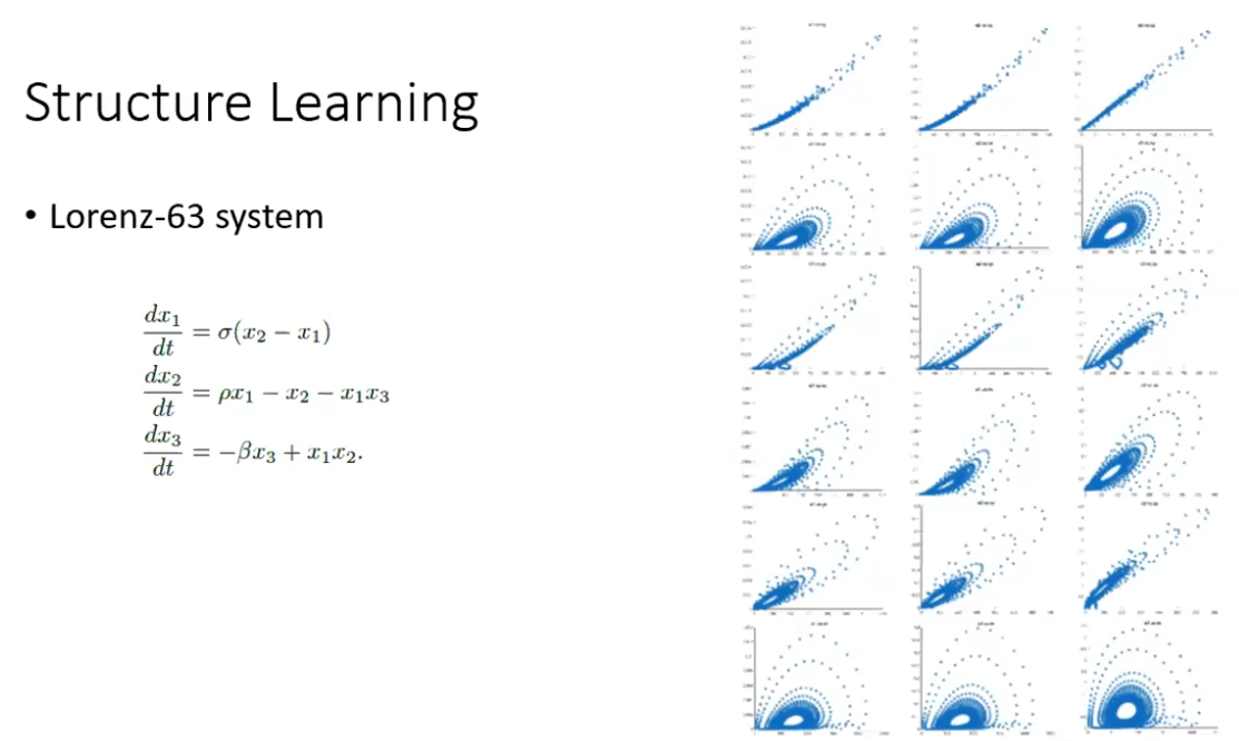
Using this very interesting library called DataDrivenDiffEq.jl that has a Koopman filters and Sparse Identification of Nonlinear Dynamics
Using the same strategy used in the Ensemble methods, we can calculate the information gain of adding each basis function and choose step by step which one to add, followed by a parameter estimation step.
(from ml20202)
what are they
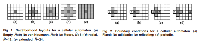
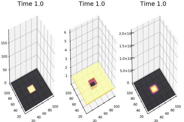
Neighborhood (from this paper)
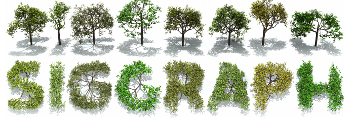
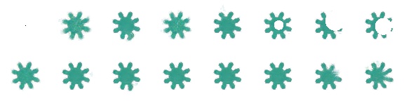
The chemical Basis of Morphogenesis
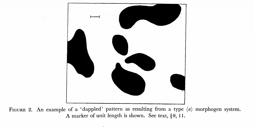
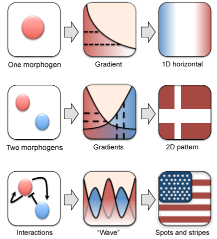
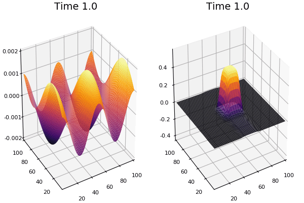
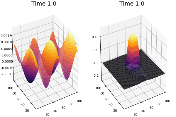
$$\frac{\delta u}{\delta t}=r_u \nabla^2u-uv^2+F(1-u)$$ $$\frac{\delta v}{\delta t}=r_v \nabla^2v+uv^2-(K+F)v$$
$$U+2V \rightarrow 3V $$ $$V \rightarrow P $$
$U$ , $V$ and P are chemical species, $u$ , $v$ are their concentrations.
$r_u$ and $r_v$ are their diffusion rates.
$K$ represents the rate of conversion of $V$ to $P$.
$F$ represents the rate of the process that feeds $U$ and drains $U$,$V$ and $P$.
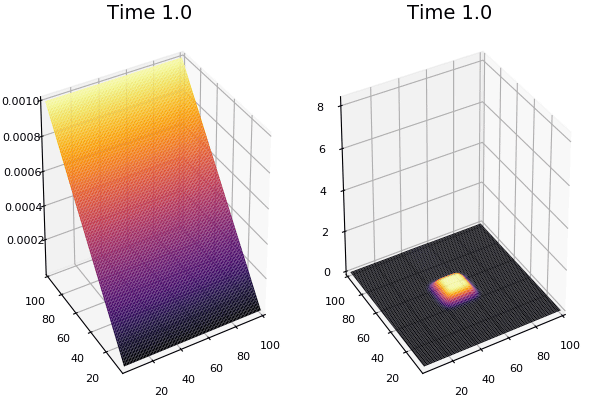
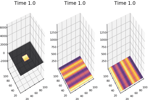
Discretized Version:
$$U'=U+(D_U \nabla^2U-UB^2+F(1-U))\Delta t$$ $$V'=V+(D_V \nabla^2V+UV^2-(K+F)V)\Delta t$$
$D_U$ & $D_V$ diffusion rates for $U$ and
$\nabla^2U$ & $\nabla^2V$ are the 2d laplacian functions
$-UV^2$ & $+UV^2$ Reaction: the chance one U and two Vs come together is $UVV$, $U$ is converted to $V$ so this amount is subtracted from A and added to B.
$F(1-U)$ feed at rate f scaled by (1-U) so it doesn't exceed 1.0
$-(K+F)$ Kill: kill rate never less than the fed rate.
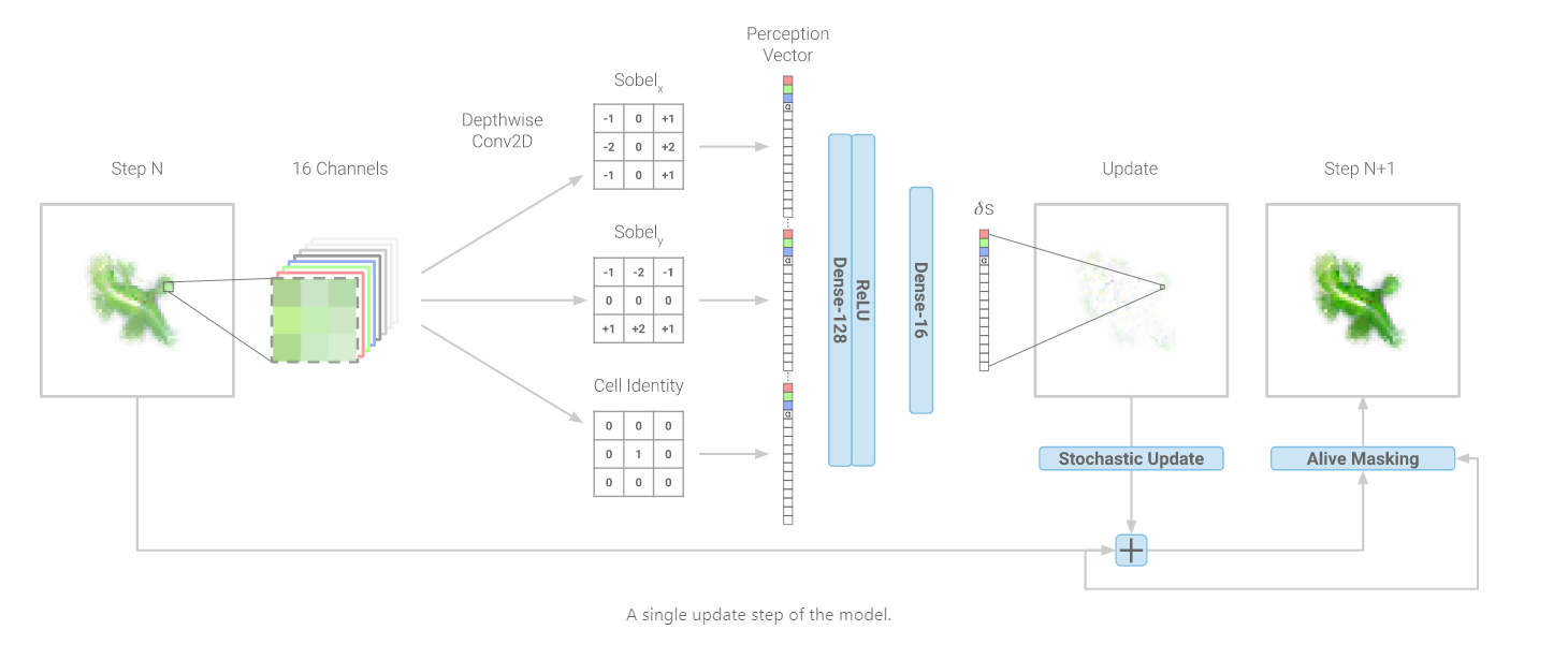
Implementation (CPU,Vectorized,GPU):
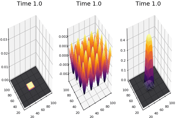
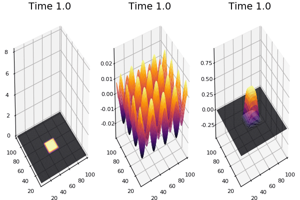
$$ \frac{\delta C}{\delta t} +(u.\nabla) c = k \nabla^2 C+f(C) $$ $$ \frac{\delta C}{\delta t} =D_C \nabla^2 C +f(C) $$
where $D_2 \nabla^2 c$ is the reaction to the neighbours and $f(c)$ is the diffusion function
The discrete form: $$ C' = C+ [D_C \nabla^2 C +f(C)] \Delta t $$
Here, $D_C$ is not constant but changes ($k$ describes the change)
$$ \frac{\delta C}{\delta t} =\nabla.(k\nabla C) +f(C) $$ $$ \nabla.(k\nabla C)=\nabla k.\nabla C+k \nabla^2C $$
$$ \nabla k.\nabla C = (D_1K)^TD_1C=k^TD_1^TD_1C$$
$$k \nabla^2C=kD_2C $$
$$ \frac{\delta C}{\delta t} =k^TD_1^TD_1C +kD_2C +f(C) $$
K structure:
$$ k=\bar{k}+U\sum{n} $$ U basis functions