RANDOM SYSTEMS
Random variables
Definition
A random variable is "a fluctuating quantity... that is described by governing equations in terms of probability distributions."
Properties:
- Not possible to predict its value
- Possible to predict the probability for seeing a given event in terms of the random variable
- Different values --> same distribution laws
Random systems
Values $x$ taken from a distribution $p(x)$. For a continuous variable:
\begin{equation*} \int_a^b p(x) \, dx \end{equation*}is the probability to observe $x$ between $a$ and $b$.
Expectation value of $f(x)$ for a continuous variable:
\begin{equation*} \left\langle f(x) \right\rangle = \lim_{N \to +\infty} \dfrac{1}{N} \sum_{i=1}^{N} f(x_i) = \int_{-\infty}^{+\infty} f(x) p(x) \, dx \end{equation*}Mean value: \begin{equation*} \overline x = \left\langle x \right\rangle = \int_{-\infty}^{+\infty} x p(x) \, dx \end{equation*}
Variance:
\begin{equation*} \sigma_{x}^{2} = \left\langle (x - \overline x)^2 \right\rangle = \left\langle x^2 \right\rangle - \left\langle x \right\rangle^2 \end{equation*}where $\left\langle x^2 \right\rangle$ is the second moment:
\begin{equation*} \left\langle x^2 \right\rangle = \int_{-\infty}^{+\infty} x^2 p(x) \, dx \end{equation*}and the standard deviation is $\sigma_{x}$.
Joint distributions
For two random variables $x$ and $y$ with a joint density $p(x, y)$, the expected value is
\begin{equation*} \left\langle f(x,y) \right\rangle = \int_{-\infty}^{+\infty} \int_{-\infty}^{+\infty} f(x,y) p(x,y) \, dx dy \end{equation*}where
\begin{equation*} \int_{-\infty}^{+\infty} \int_{-\infty}^{+\infty} p(x,y) \, dx dy \end{equation*}The probability of $x$ given $y$, $p(x|y)$ is defined by Bayes' rule
\begin{equation*} p(x|y) = \dfrac{p(x,y)}{p(y)} \end{equation*}\begin{equation*} p(belief|evidence) = \dfrac{p(evidence|belief)p(belief)}{p(evidence)} \\ posterior = \dfrac{likelihood x prior}{evidence} \end{equation*}Maximum likelihood: "The goal of maximum likelihood is to find the parameter values that give the distribution that maximise the probability of observing the data." From Medium.
INDEPENDENCE: $p(x,y) = p(x)p(y)$
PAIRS: If $y = x_1 + x_2$ for $x_1$ drawn from $p_1$, $x_2$ drawn from $p_2$ \begin{equation*} p(y) = \int_{-\infty}^{+\infty} p_1(x)p_2(y-x) \, dx = p_1(x)*p_2(x) \end{equation*}
Characteristic functions
A characteristic function is the Fourier transform of a probability distribution:
\begin{equation*} \left\langle e^{ikx} \right\rangle = \int_{-\infty}^{+\infty} e^{ikx} p(x,y) \, dx \end{equation*}The Central Limit Theorem states that in the limit $N \longrightarrow \infty$, the sum of $N$ variables approaches a Gaussian distribution:
\begin{equation*} p(y_N-\overline x) = \sqrt{\dfrac{N}{2 \pi \sigma_{x}^{2}}} e^\frac{N(y_N-\overline x)^2}{2 \sigma_{x}^{2}} \end{equation*}The cumulants $C_n$ generated by the natural logarithm of the characteristic function, written as a power series
\begin{equation*} log\left\langle e^{ikx} \right\rangle = \sum_{n=1}^{\infty} \dfrac{(ik)^n}{n!} \left\langle x^n \right\rangle \end{equation*}Entropy
The entropy of a distribution, the expected value of the information in a sample, is given by
\begin{equation*} H(x) = -\sum_{x=1}^{N} p(x) log_2p(x) \end{equation*}Stochastic processes
Including time in random systems.
Problems
6.1
(a) Work out the first three cumulants C1, C2, and C3.
The cumulants $C_n$ generated by the natural logarithm of the characteristic function, written as a power series
\begin{equation*} log\left\langle e^{ikx} \right\rangle = \sum_{n=1}^{\infty} \dfrac{(ik)^n}{n!} \left\langle x^n \right\rangle \end{equation*}
3.1 a & b
3.1 c
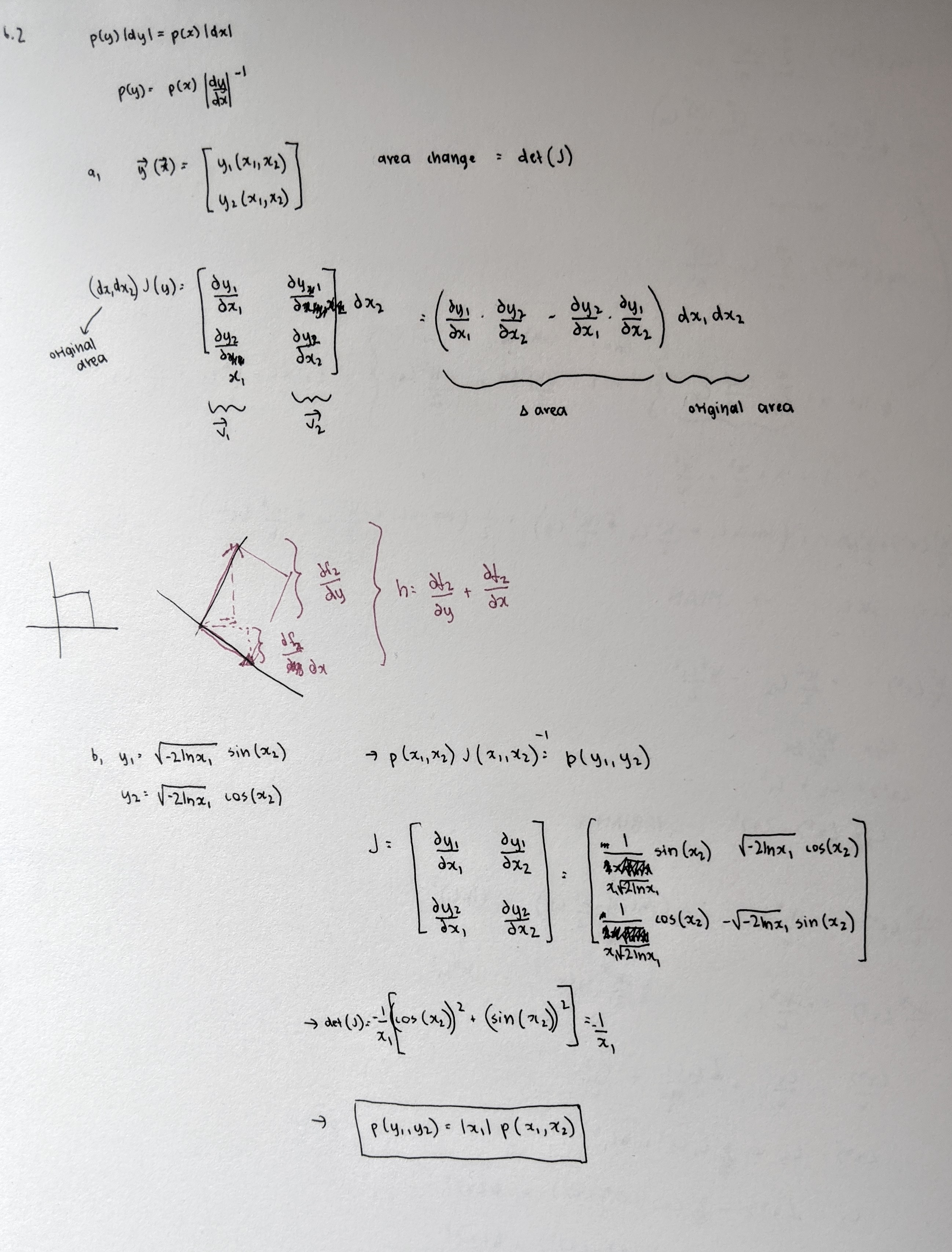
6.2
(c) Write a uniform random number generator
import numpy as np
import time
import matplotlib.pyplot as plt
%matplotlib inline

plt.rcParams['figure.figsize'] = 10, 10
class LFSR:
    def __init__(self, length, tap):
        self.length = length
        self.tap = tap

        self.a = 1103515245
        self.b = 12345
        self.c = 2 ** 31

        self.prev = self.generate_seed()
        self.string = self.generate_string()

    def generate_seed(self):
        return (self.a * int(time.time()) + self.b) % self.c

    def generate_bit(self):
        x = (self.a * self.prev + self.b) % self.c
        self.prev = x
        return float(x / self.c)

    def generate_string(self):
        #print np.array([self.generate_bit() for i in range(1000)])
        # return [float(self.generate_bit()) for i in range(self.length)]

        n = round(time.time()) % (2**self.length)
        bn = bin(int(n)).replace("0b", "")
        if len(bn) < self.length:
            fill = '00000000000'
            bn = fill[0:(self.length-len(bn))] + bn

        return bn

    def step_xor(self):
        first_item = (eval(self.string[0]) ^ eval(self.string[self.tap]))
        self.string = self.string[1:] + str(first_item)
#         return self.string
        return first_item

    def step_sum(self):
        taps = [1, 2, 3, 7]
        sum = 0

        for i in taps:
            sum += eval(self.string[i])

        first_item = sum % 2
        self.string = self.string[1:] + str(first_item)

        return first_item

    def generate_float(self):
        new_string = ''
        k = 8
        for i in range(0,k):
            new_string = new_string + str(self.step_xor())
#         print new_string
        return int(new_string, 2)
lfsr_test = LFSR(11, 8)
lfsr_test2 = LFSR(11, 8)
# print(lfsr_test.generate_string())
# print(lfsr_test.step())

# for i in range(0, 200):
#     print(lfsr_test.step_sum())

# for i in range(0, 200):
#     print("original:")
#     print(lfsr_test.generate_float())
#     print("normalized:")
#     print(lfsr_test.generate_float()/float(2**8))
N = 500

x1 = np.array([lfsr_test.generate_float()/float(2**8) for i in range(N)])
x2 = np.array([lfsr_test.generate_float()/float(2**8) for i in range(N)])

plt.scatter(x1, x2)
plt.xlabel("x1")
plt.ylabel("x2")
plt.show()
