Problem Set 3 (Random Systems)

1

(a)

Work out the first three cumulants $C_1$ , $C_2$ , and $C_3$ .

Let $x$ be any random variable. The cumulants of $x$ are defined as the coefficients $C_n$ in the following power series (in $k$ ) for the logarithm of the characteristic function. Note that $x$ doesn’t appear in the series, since it’s integrated out by the expected value.

$\sum_{n=1}^\infty \frac{(ik)^n}{n!} C_n = \log \langle e^{ikx} \rangle$

So by exponentiating each side, then expanding into a series,

$\begin{aligned} \exp \left( \sum_{n=1}^\infty \frac{(ik)^n}{n!} C_n \right) &= \langle e^{ikx} \rangle \\ \sum_{m = 0}^\infty \frac{1}{m!} \left( \sum_{n=1}^\infty \frac{(ik)^n}{n!} C_n \right)^m &= \sum_{n=0}^\infty \frac{(ik)^n}{n!} \langle x^n \rangle \end{aligned}$

This looks pretty messy, but there’s only so many places terms with low powers of $k$ can come from. To help with this, let’s expand the outer sum of the left hand side.

$1 + \sum_{n=1}^\infty \frac{(ik)^n}{n!} C_n + \frac{1}{2} \left( \sum_{n=1}^\infty \frac{(ik)^n}{n!} C_n \right)^2 + \frac{1}{6} \left( \sum_{n=1}^\infty \frac{(ik)^n}{n!} C_n \right)^3 + \ldots$

Ok, so both sides clearly start with 1. That checks out. Then to get a single power of $k$ , on the left it has to be the first term of the first series ( $m=1$ , $n=1$ ), and on the right it has to be the first term ( $n=1$ ).

$ik C_1 = ik \langle x \rangle$

So the first cumulant is $C_1 = \langle x \rangle$ , the expected value of $x$ .

To get $k^2$ , on the left we can use $m=1$ , $n=2$ or $m=2$ , $n=1$ . On the right it has to be $n=2$ .

$\begin{aligned} \frac{(ik)^2}{2} C_2 + \frac{1}{2} (ik C_1)^2 &= \frac{(ik)^2}{2} \langle x^2 \rangle \\ C_2 &= \langle x^2 \rangle - C_1^2 \\ C_2 &= \langle x^2 \rangle - \langle x \rangle^2 \end{aligned}$

This is the variance of $x$ .

For $k^3$ , there are three relevant terms from the left hand side: $m=1$ , $n=3$ ; $m=2$ , the product of $n=1$ and $n=2$ (this happens two ways so we pick up a factor of 2); and $m=3$ , $n=1$ .

$\begin{aligned} \frac{(ik)^3}{6} C_3 + 2 \frac{1}{2} ik C_1 \frac{(ik)^2}{2} C_2^2 + \frac{1}{6} (ik C_3)^3 &= \frac{(ik)^3}{6} \langle x^3 \rangle \\ C_3 + 3 C_1 C_2 + C_1^3 = \langle x^3 \rangle \\ C_3 = \langle x^3 \rangle - 3 C_1 C_2 - C_1^3 \\ C_3 = \langle x^3 \rangle - 3 \langle x \rangle \langle x^2 \rangle + 2 \langle x \rangle^3 \end{aligned}$

which is the third central moment of $x$ .

Stopping here is a little misleading, since fourth and higher order cumulants are not equal to the corresponding central moments. So it goes.

(b)

Evaluate the first three cumulants for a Gaussian distribution.

Ok, time to integrate. I’ll start with some basic facts and work my way up from there.

First, the Gaussian distribution is normalized.

$\int_{-\infty}^\infty \frac{1}{\sqrt{2 \pi \sigma^2}} e^{-(x - \mu)^2/(2 \sigma^2)} dx = 1$

If you want to verify this yourself, there are a lot of ways to do it.

Next, the mean of a Gaussian distribution with $\mu = 0$ is 0. This follows from finding an explicit antiderivative.

$\begin{aligned} \langle N(0, \sigma^2) \rangle &= \int_{-\infty}^\infty \frac{1}{\sqrt{2 \pi \sigma^2}} x e^{-x^2/(2 \sigma^2)} dx \\ &= \frac{1}{\sqrt{2 \pi \sigma^2}} \int_{-\infty}^\infty \frac{d}{dx} \left[ -\sigma^2 e^{-x^2/(2 \sigma^2)} \right] dx \\ &= \frac{1}{\sqrt{2 \pi \sigma^2}} \left[ -\sigma^2 e^{-x^2/(2 \sigma^2)} \right]_ {-\infty}^\infty \\ &= 0 \end{aligned}$

There’s also a shortcut we could have taken here: $x$ is an odd function, while $N(0, \sigma^2)$ is even. So their product is an odd function, and the integral across the whole real line has to be zero. But we’ll use the antiderivative above in other contexts, so I wanted to work it out fully.

Then the fact that the mean of a general Gaussian distribution is $\mu$ follows from a simple change of variables.

$\begin{aligned} \langle N(\mu, \sigma^2) \rangle &= \int_{-\infty}^\infty \frac{1}{\sqrt{2 \pi \sigma^2}} x e^{-(x - \mu)^2/(2 \sigma^2)} dx \\ &= \int_{-\infty}^\infty \frac{1}{\sqrt{2 \pi \sigma^2}} (x + \mu) e^{-x^2/(2 \sigma^2)} dx \\ &= \int_{-\infty}^\infty \frac{1}{\sqrt{2 \pi \sigma^2}} x e^{-x^2/(2 \sigma^2)} dx + \mu \int_{-\infty}^\infty \frac{1}{\sqrt{2 \pi \sigma^2}} e^{-x^2/(2 \sigma^2)} dx \\ &= \langle N(0, \sigma^2) \rangle + \mu \\ &= \mu \end{aligned}$

Next, we can integrate by parts to show that $\langle N(0, \sigma^2)^2 \rangle$ is $\sigma^2$ . This uses the same antiderivative we found earlier.

$\begin{aligned} \langle N(0, \sigma^2)^2 \rangle &= \int_{-\infty}^\infty \frac{1}{\sqrt{2 \pi \sigma^2}} x^2 e^{-x^2/(2 \sigma^2)} dx \\ &= \frac{1}{\sqrt{2 \pi \sigma^2}} \int_{-\infty}^\infty x \left( x e^{-x^2/(2 \sigma^2)} \right) dx \\ &= \frac{1}{\sqrt{2 \pi \sigma^2}} \left( \left[ x (-\sigma^2 e^{-x^2/(2 \sigma^2)}) \right]_ {-\infty}^\infty -\int_{-\infty}^\infty -\sigma^2 e^{-x^2/(2 \sigma^2)} dx \right) \\ &= \sigma^2 \end{aligned}$

So, using a change of variables again,

$\begin{aligned} \langle N(\mu, \sigma^2)^2 \rangle &= \int_{-\infty}^\infty \frac{1}{\sqrt{2 \pi \sigma^2}} x^2 e^{-(x - \mu)^2/(2 \sigma^2)} dx \\ &= \int_{-\infty}^\infty \frac{1}{\sqrt{2 \pi \sigma^2}} (x + \mu)^2 e^{-x^2/(2 \sigma^2)} dx \\ &= \int_{-\infty}^\infty \frac{1}{\sqrt{2 \pi \sigma^2}} (x^2 + 2x \mu + \mu^2) e^{-x^2/(2 \sigma^2)} dx \\ &= \langle N(0, \sigma^2)^2 \rangle + 2 \mu \langle N(0, \sigma^2) \rangle + \mu^2 \\ &= \sigma^2 + \mu^2 \end{aligned}$

To compute $\langle N(0, \sigma^2)^3 \rangle$ , we could integrate by parts again (using $u = x^2$ and $v = x e^{-x^2/(2\sigma^2)}$ ). But instead I’ll just note that $x^3$ is an odd function, so

$\begin{aligned} \langle N(0, \sigma^2)^3 \rangle &= \int_{-\infty}^\infty \frac{1}{\sqrt{2 \pi \sigma^2}} x^3 e^{-x^2/(2 \sigma^2)} dx \\ &= 0 \end{aligned}$

Thus

$\begin{aligned} \langle N(\mu, \sigma^2)^3 \rangle &= \int_{-\infty}^\infty \frac{1}{\sqrt{2 \pi \sigma^2}} x^3 e^{-(x - \mu)^2/(2 \sigma^2)} dx \\ &= \int_{-\infty}^\infty \frac{1}{\sqrt{2 \pi \sigma^2}} (x + \mu)^3 e^{-x^2/(2 \sigma^2)} dx \\ &= \int_{-\infty}^\infty \frac{1}{\sqrt{2 \pi \sigma^2}} (x^3 + 3 \mu x^2 + 3 \mu^2 x + \mu^3) e^{-x^2/(2 \sigma^2)} dx \\ &= \langle N(0, \sigma^2)^3 \rangle + 3\mu \langle N(0, \sigma^2)^2 \rangle + 3\mu^2 \langle N(0, \sigma^2) \rangle + \mu^3 \\ &= 3 \mu \sigma^2 + \mu^3 \end{aligned}$

We’re finally ready to plug things together.

$\begin{aligned} C_1 &= \langle x \rangle \\ &= \mu \\ C_2 &= \langle x^2 \rangle - \langle x \rangle^2 \\ &= (\sigma^2 + \mu^2) - \mu^2 \\ &= \sigma^2 \\ C_3 &= \langle x^3 \rangle - 3 \langle x \rangle \langle x^2 \rangle + 2 \langle x \rangle^3 \\ &= (3 \mu \sigma^2 + \mu^3) -3 \mu (\sigma^2 + \mu^2) + 2 \mu^3 \\ &= 0 \end{aligned}$

It turns out all higher order cumulants of the Gaussian distribution are also zero, and it is the only distribution with this property.

2

(a)

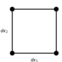
If $\overrightharpoon{y}(\overrightharpoon{x}) = (y_1(x_1, x_2), y_2(x_1, x_2))$ is a coordinate transformation, what is the area of a differential element $dx_1 dx_2$ after it is mapped into the $\overrightharpoon{y}$ plane?

The transformation sends a differential element like this

differential square

to a parallelogram like this

differential square

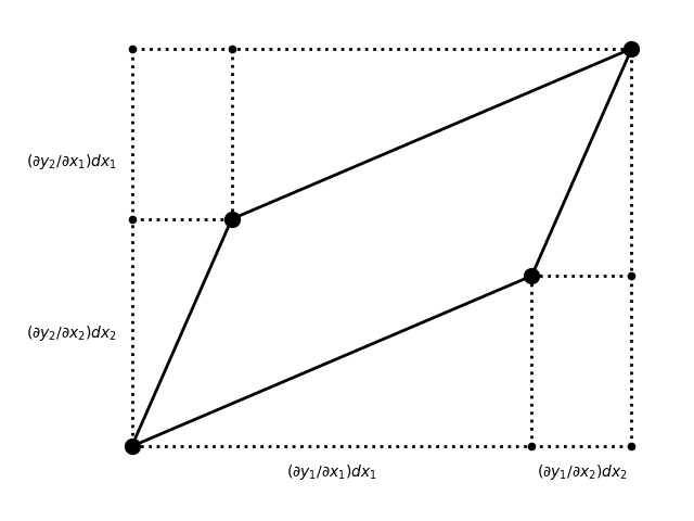
The area of the box containing the parallelogram is

$\left( \frac{\partial y_1}{\partial x_1} dx_1 + \frac{\partial y_1}{\partial x_2} dx_2 \right) \left( \frac{\partial y_2}{\partial x_1} dx_1 + \frac{\partial y_2}{\partial x_2} dx_2 \right)$

And the area of the triangles and rectangles drawn in dotted lines is

$\frac{\partial y_1}{\partial x_1} dx_1 \frac{\partial y_2}{\partial x_1} dx_1 + \frac{\partial y_1}{\partial x_2} dx_2 \frac{\partial y_2}{\partial x_2} dx_2 + 2 \frac{\partial y_1}{\partial x_2} dx_2 \frac{\partial y_2}{\partial x_1} dx_1$

Thus the area of the parallelogram is their difference:

$\frac{\partial y_1}{\partial x_1} dx_1 \frac{\partial y_2}{\partial x_2} dx_2 - \frac{\partial y_1}{\partial x_2} dx_2 \frac{\partial y_2}{\partial x_1} dx_1$

The factor of area change is the absolute value of the determinant of the Jacobian matrix of $\overrightharpoon{y}$ . (The sign tells us if the handedness of the coordinate system was flipped.)

(b)

Let

$\begin{aligned} y_1 &= \sqrt{-2 \ln x_1} \sin(x_2) \\ y_2 &= \sqrt{-2 \ln x_1} \cos(x_2) \\ \end{aligned}$

If $p(x_1, x_2)$ is uniform, what is $p(y_1, y_2)$ ?

The probability density at a point $y_1, y_2$ is

$p(y_1, y_2) = p(x_1(y_1, y_2), x_2(y_1, y_2)) \left| \det[\bold{J}^{-1}(y_1, y_2)] \right|$

So let’s invert the transform. By squaring and adding both sides, we find that

$\begin{aligned} y_1^2 + y_2^2 &= -2 \ln x_1 (\sin(x_2)^2 + \cos(x_2)^2) \\ &= -2 \ln x_1 \\ x_1 &= e^{-(y_1^2 + y_2^2)/2} \end{aligned}$

By dividing the first equation by the second,

$\begin{aligned} \frac{y_1}{y_2} &= \frac{\sin(x_2)}{\cos(x_2)} \\ x_2 &= \tan^{-1} \left( \frac{y_1}{y_2} \right) \end{aligned}$

So $x_1$ is determined by the radius of the transformed sample, and $x_2$ is determined by its angle. If we sample $x_1$ between 0 and 1, we’ll get radii between 0 and infinity, and if we sample $x_2$ between 0 and $2 \pi$ , we’ll cover all angles in $y$ space. This region of $x$ space has area $2 \pi$ , so the probability density $p(x_1, x_2)$ will be uniformly $1 / (2 \pi)$ .

So the Jacobian matrix of this (inverse) transformation is

$\begin{aligned} \bold{J}^{-1} &= \begin{bmatrix} \frac{\partial x_1}{\partial y_1} & \frac{\partial x_1}{\partial y_2} \\ \frac{\partial x_2}{\partial y_1} & \frac{\partial x_2}{\partial y_2} \end{bmatrix} \\ &= \begin{bmatrix} -y_1 e^{-(y_1^2 + y_2^2)/2} & -y_2 e^{-(y_1^2 + y_2^2)/2} \\ \frac{y2}{y_1^2 + y_2^2} & \frac{-y1}{y_1^2 + y_2^2} \end{bmatrix} \end{aligned}$

And

$\left| \det[\bold{J}^{-1}] \right| = e^{-(y_1^2 + y_2^2)/2}$

Putting the pieces together,

$\begin{aligned} p(y_1, y_2) &= p(x_1(y_1, y_2), x_2(y_1, y_2)) \left| \det[\bold{J}^{-1}(y_1, y_2)] \right| \\ &= \frac{1}{2 \pi} e^{-(y_1^2 + y_2^2)/2} \end{aligned}$

This is the two dimensional normal normal distribution with mean $(0, 0)$ and identity covariance matrix.

(c)

Write a uniform random number generator, and transform it by the equations above. Numerically evaluate the first three cumulants of its output.

I implemented a 64 bit xorshift random number generator (code lives here). These generators are mathematically equivalent to LFSRs, but they are more efficient to implement in software. I got the special constants from Numerical Recipes in C, third edition.

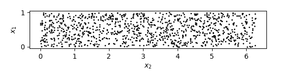
First, let’s make sure it works. Here are 1,000 samples drawn from a uniform distribution on a rectangle of area $2 \pi$ .

uniform samples

And here are the transformed samples.

gaussian samples

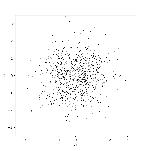
Looks good to me.

Cumulants can be defined for multivariate distributions, but since I already worked out the univariate cases above I’m just going to calculate them for $y_1$ alone. I computed $\langle y_1 \rangle$ , $\langle y_1^2 \rangle$ , and $\langle y_1^3 \rangle$ experimentally by taking the average over a large sample of $y_1$ , $y_1^2$ , and $y_1^3$ , respectively. Then I just plugged the resulting values into the formulas I found in the previous problem.

With 100,000 samples, I get these values.

$\begin{aligned} C_1 &= 0.00106 \\ C_2 &= 1.00525 \\ C_3 &= -0.00516 \end{aligned}$

With 1,000,000 samples, I get these.

$\begin{aligned} C_1 &= 7.524 \times 10^{-5} \\ C_2 &= 0.9992 \\ C_3 &= -0.003815 \end{aligned}$

And with one hundred million samples, I get these.

$\begin{aligned} C_1 &= 8.541 \times 10^{-5} \\ C_2 &= 0.9999 \\ C_3 &= 4.013 \times 10^{-4} \end{aligned}$

These are consistent with the predicted values.

3

(a)

For an order 4 maximal LFSR write down the bit sequence.

Using taps one and four generates a maximum length bit sequence. I wrote a simple Python program to compute the values for me. The columns are $x_{n-1}$ , $x_{n-2}$ , $x_{n-3}$ , and $x_{n-4}$ .

[0 0 0 1]
[1 0 0 0]
[1 1 0 0]
[1 1 1 0]
[1 1 1 1]
[0 1 1 1]
[1 0 1 1]
[0 1 0 1]
[1 0 1 0]
[1 1 0 1]
[0 1 1 0]
[0 0 1 1]
[1 0 0 1]
[0 1 0 0]
[0 0 1 0]

(b)

If an LFSR has a clock rate of 1 GHz, how long must the register be for the time between repeats to be the age of the universe (~ $10^{10}$ years)?

A maximal LFSR of order $n$ has a cycle of length $2^n - 1$ . There are $3.17 \times 10^8$ seconds in a year.

$\begin{aligned} 2^n - 1 &= 10^{10} \cdot 3.17 \times 10^8 \cdot 10^9 \\ 2^n - 1 &= 3.17 \times 10^{27} \\ n &= \log_2(3.17 \times 10^{27} + 1) \\ n &\approx 91.4 \end{aligned}$

So you’d need 92 bits to exceed the age of the universe.

I used Wolfram Alpha to compute the logarithm above, but we can also estimate it ourselves. Recall that $2^{10} \approx 10^3$ , so to change from base 10 to base 2 we just need to multiply the exponent by about 3.

$\begin{aligned} n &= \log_2(3.17 \times 10^{27} + 1) \\ n &\approx \log_2(10^{27}) \\ n &\approx \log_2(2^{81}) \\ n &\approx 81 \end{aligned}$

This is a little under the real answer since I multiplied the exponent by 3 rather than $10/3$ . But order of magnitude wise it’s completely fine.

4

(a)

Use a Fourier transform to solve the diffusion equation (assume that the initial condition is a normalized delta function at the origin).

For reference, the diffusion equation is

$\frac{\partial p}{\partial t}(x, t) = D \frac{\partial^2 p}{\partial x^2}(x, t)$

There are two different conventions about where to stick the constants in the definition of the Fourier transform; I will use the one in my handy Fourier transform notes.

Taking the Fourier transform of both sides with respect to $x$ , we find

$\begin{aligned} \frac{\partial \hat{p}}{\partial t}(f, t) &= (2 \pi i f)^2 D \hat{p}(f, t) \\ &= -(2 \pi f)^2 D \hat{p}(f, t) \end{aligned}$

Recall that the Fourier transform of a derivative just picks up a factor of $2 \pi i f$ (this is derived in my Fourier transform notes).

Let’s try the ansatz $\hat{p}(f, t) = A e^{-\lambda t}$ .

$\begin{aligned} -\lambda A e^{-\lambda t} &= -(2 \pi f)^2 D A e^{-\lambda t} \\ \lambda &= (2 \pi f)^2 D \end{aligned}$

So $\hat{p}(f, t) = A e^{-(2 \pi f)^2 D t}$ . Now if $p(x, 0)$ is a normalized delta function, then $\hat{p(f, 0)}$ is uniformly 1. Thus $A = 1$ .

$\hat{p}(f, t) = e^{-(2 \pi f)^2 D t}$

As derived in my Fourier transform notes, this is the transform of a Gaussian with zero mean and variance $\sigma^2 = 2 D t$ . Thus

$p(x, t) = \frac{1}{\sqrt{4 \pi D t}} e^{-x^2 / (4Dt)}$

(b)

What is the variance as a function of time?

We already demonstrated that $p(x, t)$ is a Gaussian with zero mean and variance $\sigma^2 = 2 D t$ . So the variance grows linearly over time.

(c)

How is the diffusion coefficient for Brownian motion related to the viscosity of a fluid?

In the chapter we found that

$\langle x^2 \rangle = \frac{kT}{3 \pi \mu a} t$

Thus, assuming an isotropic and homogeneous fluid, the variance of the particle’s position in the fluid is also $kT / (3 \pi \mu a) t$ , since $\langle x \rangle^2$ will be zero.

$\begin{aligned} \sigma^2 &= \langle x^2 \rangle - \langle x \rangle^2 \\ &= \langle x^2 \rangle \\ &= \frac{kT}{3 \pi \mu a} t \end{aligned}$

To model a particle of the fluid with Brownian motion we’ll need to match variances.

$\begin{aligned} 2 D t &= \frac{kT}{3 \pi \mu a} t \\ D &= \frac{kT}{6 \pi \mu a} \end{aligned}$

(d)

Write a program (including the random number generator) to plot the position as a function of time of a random walker in 1D that at each time step has an equal probability of making a step of $\pm 1$ . Plot an ensemble of 10 trajectories, each 1000 points long, and overlay error bars of width $3\sigma(t)$ on the plot.

I used the same random number generator as in the previous problem to draw uniform samples from $\{-1, 1\}$ . The trajectories are simply sums of these random variables.

In the chapter we found that the diffusion constant for Brownian motion is $\langle \delta^2 \rangle / (2 \tau)$ . In this case the expected value of $\delta^2$ is 1, since all possible values of the random variable squared are one ( $(-1)^2 = 1^2 = 1$ ). Our timestep $\tau$ is also $1$ . So $D = 1/2$ . Thus $\sigma^2 = t$ , and $\sigma = \sqrt{t}$ .

random walk

(e)

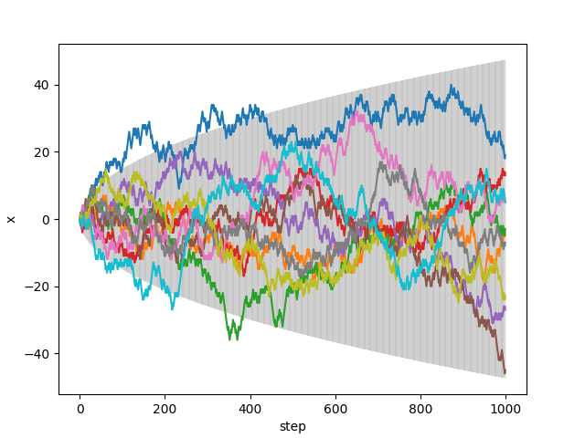
What fraction of the trajectories should be contained in the error bars?

At any given timestep, the positions of the trajectories are normally distributed with variance $t$ . So 87% of the trajectories should be within 1.5 standard deviations of the mean. This value can be computed as

$\int_{1.5 t}^{1.5 t} \frac{1}{\sqrt{2 \pi t}} e^{-x^2/(2t)} dx \approx 0.8664$

Alternatively, you can look it up like I did in a standard normal table.

However there’s another way to interpret this question. Let’s try to find the probability that a trajectory has never left the error bars. More formally, we want to know the probability that we end in state $k$ and never left the error bars along the way, for each time step $t_n$ . Let’s call this probability $q_n(k)$ .

To start, though, let’s answer a simpler question: how many different paths reach state $k$ at time step $n$ ? I’ll call this number $N_n(k)$ . If we go back one step in time, there’s only two states a path could have stepped from to get to $k$ : $k-1$ and $k+1$ . So $N_n(k)$ satisfies the recurrence relation

$N_n(k) = N_{n-1}(k-1) + N_{n-1}(k+1)$

This just describes Pascal’s triangle. Thus the number of paths that reach state $k$ at time step $n$ is exactly $n$ choose $k$ .

$\begin{matrix} k = 5 & & & & & & 1 & \\ k = 4 & & & & & 1 & & \\ k = 3 & & & & 1 & & 5 & \\ k = 2 & & & 1 & & 4 & & \\ k = 1 & & 1 & & 3 & & 10 & \\ k = 0 & 1 & & 2 & & 6 & & \ldots \\ k = -1 & & 1 & & 3 & & 10 & \\ k = -2 & & & 1 & & 4 & & \\ k = -3 & & & & 1 & & 5 & \\ k = -4 & & & & & 1 & & \\ k = -5 & & & & & & 1 & \\ &t_0&t_1&t_2&t_3&t_4&t_5&\ldots \end{matrix}$ $N_n(k) = {n \choose k} = \frac{n!}{k!(n-k)!}$

Note that the total number of paths at time step $n$ is $2^n$ . Fundamentally this is true because each path splits in two at each time step, but you can also sanity check it by summing the columns of the triangle above. Given this, the probability of reaching state $k$ at time step $n$ has to be $n$ choose $k$ divided by $2^n$ :

$p_n(k) = \frac{1}{2^n}{n \choose k} = \frac{1}{2^n} \frac{n!}{k!(n-k)!}$

This ensures that

$\sum_{k=-\infty}^\infty p_n(k) = 1$

for all $n$ .

Unfortunately this expression for $p_n(k)$ is hard to compute directly, since both the numerator and denominator quickly become unreasonably large. And there’s no simple cancellation of terms that would let us compute the result without enormous intermediate values.

But the recurrence relation that led us to $N_n(k)$ can easily be modified to describe $p_n(k)$ : just multiply by $1/2$ at each step. This ensures the normalization factor of $2^n$ is taken into account.

$\begin{aligned} p_0(k) &= \begin{cases} 1 &\text{if } k = 0 \\ 0 &\text{if } k \neq 0 \end{cases} \\ p_n(k) &= \frac{1}{2} \left( p_{n-1}(k-1) + p_{n-1}(k+1) \right) \end{aligned}$

Visually, this amounts to filling in this triangle of probabilities from left to right. Each number is simply the sum of the two immediately before it, divided by two. All the columns sum to one.

$\begin{matrix} k = 5 & & & & & & 1/32 & \\ k = 4 & & & & & 1/16 & & \\ k = 3 & & & & 1/8 & & 5/32 & \\ k = 2 & & & 1/4 & & 1/4 & & \\ k = 1 & & 1/2 & & 3/8 & & 5/16 & \\ k = 0 & 1 & & 1/2 & & 3/8 & & \ldots \\ k = -1 & & 1/2 & & 3/8 & & 5/16 & \\ k = -2 & & & 1/4 & & 1/4 & & \\ k = -3 & & & & 1/8 & & 5/32 & \\ k = -4 & & & & & 1/16 & & \\ k = -5 & & & & & & 1/32 & \\ &p_0(k)&p_1(k)&p_2(k)&p_3(k)&p_4(k)&p_5(k)&\ldots \end{matrix}$

We can use a similar technique to calculate what we really want: $q_n(k)$ , i.e. the probability of reaching state $k$ at time step $n$ and never having gone outside the error bars along the way. All we need to do is zero out the probabilities that fall outside our bounds.

$\begin{matrix} k = 5 & & & & & & 0 & \\ k = 4 & & & & & 0 & & \\ k = 3 & & & & 0 & & 3/32 & \\ k = 2 & & & 1/4 & & 3/16 & & \\ k = 1 & & 1/2 & & 3/8 & & 9/32 & \\ k = 0 & 1 & & 1/2 & & 3/8 & & \ldots \\ k = -1 & & 1/2 & & 3/8 & & 9/32 & \\ k = -2 & & & 1/4 & & 3/16 & & \\ k = -3 & & & & 0 & & 3/32 & \\ k = -4 & & & & & 0 & & \\ k = -5 & & & & & & 0 & \\ &p_0(k)&p_1(k)&p_2(k)&p_3(k)&p_4(k)&p_5(k)&\ldots \end{matrix}$

The columns no longer sum to one, since not all paths that reach in bounds states never went out of bounds beforehand. For reference, here are the standard deviation bounds relevant for the figure above.

n	1.5 * sqrt(n)
1	1.5
2	2.1
3	2.6
4	3.0
5	3.4

Because nonzero probabilities never occur outside $k > 1.5 \sqrt{n}$ , this technique is surprisingly scalable. For instance, there are only 95 nonzero values in the 1,000th column. (Contrast this with $N_{1000}(k)$ , for which there would be 2001 nonzero values, many of which are astronomically large.)

This makes it easy to compute the values for all $n$ up to 1,000.

probs

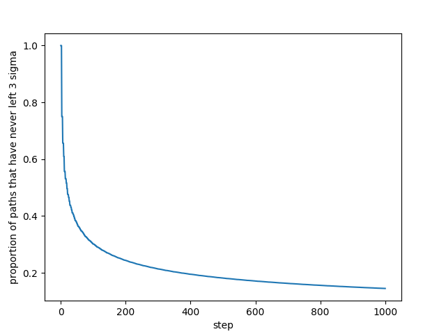
And to answer the specific question we started with, 14.5% of all possible trajectories have never left $\pm1.5 \sigma$ at step 1000.