Problem Set 4 (Numeric ODEs)

1

What is the second-order approximation error of the Heun method, which averages the slope at the beginning and the end of the interval?

Let’s expand $f$ , viewed as a function of $h$ .

$\begin{aligned} y(x + h) &= y(x) + \frac{h}{2} \left( f(x, y(x)) + f(x + h, y(x) + f(x, y(x))) \right) \\ &= y(x) + \frac{h}{2} f(x, y(x)) + \frac{h}{2} f(x + h, y(x) + f(x, y(x))) \\ &= y(x) + \frac{h}{2} f(x, y(x)) \\ &\hphantom{= } + \frac{h}{2} \left( f(x, y(x)) + h \left( \frac{\partial f}{\partial x} + f(x, y(x)) \frac{\partial f}{\partial y}) \right) + \mathcal{O}(h^2) \right) \\ &= y(x) + h f(x, y(x)) + \frac{h^2}{2} \left( \frac{\partial f}{\partial x} + f(x, y(x)) \frac{\partial f}{\partial y}) \right) + \mathcal{O}(h^3) \end{aligned}$

This agrees with the ideal Taylor expansion given in the chapter, so the Heun method is accurate to second order.

2

For a simple harmonic oscillator $\ddot{y} + y = 0$ , with initial conditions $y(0) = 1$ , $\dot{y}(0) = 0$ , find $y(t)$ from $t = 0$ to $100 \pi$ . Use an Euler method and a fixed-step fourth-order Runge–Kutta method. For each method check how the average local error, and the error in the final value and slope, depend on the step size.

I implemented Euler, RK4, and adaptive RK4 integrators in C++. Code lives here.

The integrators solve problems of the form

$\frac{dy}{dx} = f(x, y)$

So we have to manipulate the problem a bit in order to get it to fit. Specifically, we need to transform the given second order ODE into a system of first order ODEs. To do so, define two functions $y_0(x)$ and $y_1(x)$ . The former will be equal to the original $y$ , and the latter will be equal to $\dot{y}$ (so $\dot{y_1} = \ddot{y} = -y$ ).

$\begin{bmatrix} \dot{y_0}(x) \\ \dot{y_1}(x) \end{bmatrix} = \begin{bmatrix} y_1(x) \\ -y_0(x) \end{bmatrix}$

Thus we can solve a two variable system where $f(x, (y_0, y_1)) = (y_1, -y_0)$ .

Next, a few notes on how I’m measuring error. The analytic solution for the specified initial conditions is $y(x) = \sin(x)$ . We can compare against this to compute global error. For local error, though, this won’t work. Comparing against $\sin(x)$ for intermediate values of $x$ would give the cumulative error up to that point, whereas we want to assume that the last position was completely accurate and see how far we’ve diverged in just the last step. To do this, we can use the general solution.

$y(x) = A \cos(x) + B \sin(x)$

The coefficients are easy to find given a set of initial conditions: $A = y(0)$ and $B = \dot{y}(0)$ . So to compute the local error for each step, the right procedure is to take the last point $(y_0(x), y_1(x))$ we found (the one we’re stepping from), fit the general solution to it $y(x + h) = y_0(x) \cos(h) + y_1(x) \sin(h)$ , then compute the local error at $x + h$ as

$y_0(x + h) - y(x + h) = y_0(x + h) - y_0(x) \cos(h) - y_1(x) \sin(h)$

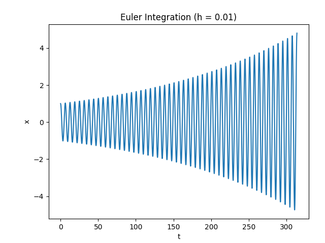
Ok, on to the results. Qualitatively, with a time step of 0.01, the Euler integrator grows exponentially.

euler trajectory

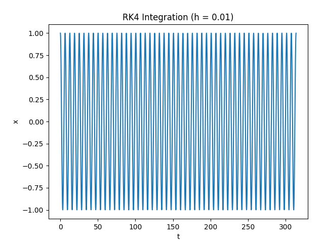
Meanwhile the RK4 integrator preserves the amplitude.

rk4 trajectory

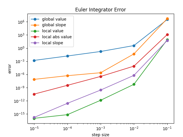
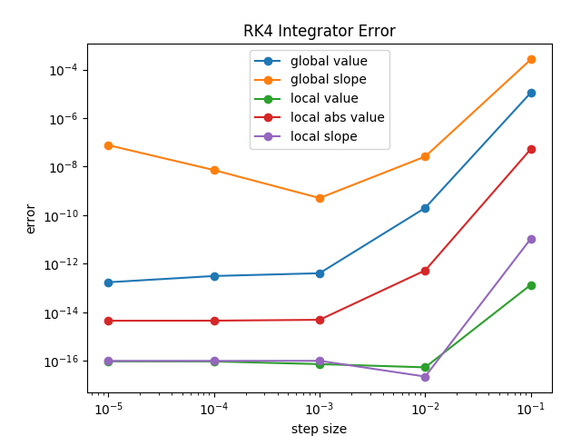
Here is how the errors of the two integrators stack up. The errors of the RK4 integrator are, generally speaking, much lower for a given step size. Interestingly, the RK4 error in slope starts to rise as the step size goes below $10^{-3}$ . Presumably this is due to accumulation of roundoff error.

euler error

rk4 error

3

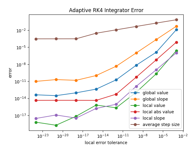
Write a fourth-order Runge–Kutta adaptive stepper for the preceding problem, and check how the average step size that it finds depends on the desired local error.

For my adaptive stepper, I multiply the step size by 0.8 if the error estimate is greater than the threshold, and multiply it by 1.2 if the error estimate is less than half the threshold. (It’s important that $0.8 \times 1.2 \neq 1$ , so that the step size can get arbitrarily close to any value with enough iterations.) For the error estimate, I’m looking at the absolute value of the value error (slope is ignored). I use the result generated by the two half steps, since it should be more accurate than the single full step.

ark4 error

4

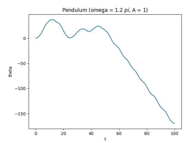
Numerically solve the differential equation describing a pendulum attached to a platform that moves along the z axis:

$l \ddot{\theta} + (g + \ddot{z}) \sin(\theta) = 0$

Take the motion of the platform to be periodic, and interactively explore the dynamics of the pendulum as a function of the amplitude and frequency of the excitation.

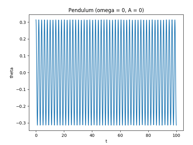
For this problem I used the adaptive step RK4 integrator, with a local error tolerance of $10^{-8}$ . I defined the pendulum length to be 1 meter, and let $g$ have its normal value of 9.8 meters per second squared. I moved the platform according to $z(t) = A \cos(\omega t)$ , and explored different values of $A$ and $\omega$ (amplitude and frequency).

When the platform doesn’t move at all, the motion is regular and periodic as expected.

pendulum 1

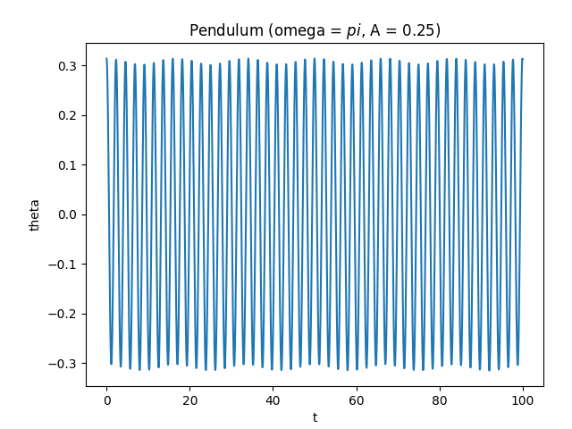
When the platform only moves a bit, the motion is subtly altered.

pendulum 2

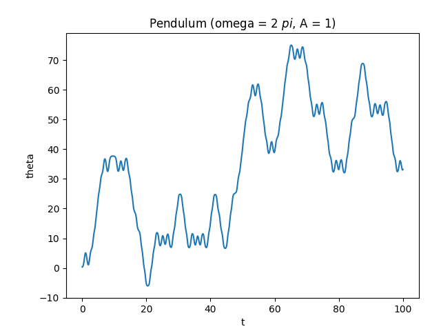
But when the movement is more intense, more interesting behavior can emerge. Here the movement of the platform excites a resonance in the pendulum system, leading to the pendulum being swung around at a roughly constant rate.

pendulum 3

Here the pendulum swings chaotically.

pendulum 4