Problem Set 6 (FEM)

1

Consider the damped wave equation

$\frac{\partial^2 u}{\partial t^2} = v^2 \frac{\partial^2 u}{\partial x^2} + \gamma \frac{\partial}{\partial t} \frac{\partial^2 u}{\partial x^2}$

Take the solution domain to be the interval [0, 1].

(a)

Use the Galerkin method to find an approximating system of differential equations.

We will search for an approximate solution of the form

$u(x, t) = \sum_{i=1}^n a_i(t) \varphi_i(x)$

(where $n$ is yet to be determined). From here on out I will just write $a_i$ and $\varphi_i$ ; it is understood that these are functions of time and space, respectively. Thus the damped wave equation becomes

$\sum_{i=1}^n \left( \frac{d^2 a_i}{d t^2} \varphi_i - v^2 a_i \frac{d^2 \varphi_i}{d x^2} - \gamma \frac{d a_i}{d t} \frac{d^2 \varphi_i}{d x^2} \right) = 0$

For each basis function $\varphi_i$ , we construct a Galerkin constraint

$\begin{aligned} 0 &= \int_0^1 \sum_{j=1}^n \left( \frac{d^2 a_j}{d t^2} \varphi_j - v^2 a_j \frac{d^2 \varphi_j}{d x^2} - \gamma \frac{d a_j}{d t} \frac{d^2 \varphi_j}{d x^2} \right) \varphi_i dx \\ &= \sum_{j=1}^n \left( \frac{d^2 a_j}{d t^2} \int_0^1 \varphi_j \varphi_i dx - \left(v^2 a_j + \gamma \frac{d a_j}{d t} \right) \int_0^1 \frac{d^2 \varphi_j}{d x^2} \varphi_i dx \right) \\ \end{aligned}$

This may be written as

$\bold{A} \frac{d^2 \overrightharpoon{a}}{d t^2} - \gamma \bold{B} \frac{d \overrightharpoon{a}}{d t} - v^2 \bold{B} \overrightharpoon{a} = 0$

where

$\begin{aligned} \bold{A}_{i, j} &= \int_0^1 \varphi_i \varphi_j dx \\ \bold{B}_{i, j} &= \int_0^1 \varphi_i \frac{d^2 \varphi_j}{d x^2} dx \\ &= \left[ \varphi_i \frac{d \varphi_j}{d x} \right]_ {0}^1 - \int_0^1 \frac{d \varphi_i}{dx} \frac{d \varphi_j}{dx} dx \\ \end{aligned}$

This gives a system of second order linear homogeneous ODEs.

Note that I integrated $\bold{B}$ by parts in order to reduce the order of the highest order derivative of $\varphi_j$ that appears. Practically speaking, this lets us use lower order basis functions, since we can let the higher derivatives be zero. This may seem like cheating — after all, the two expressions are equal, so integrating by parts shouldn’t magically make $\bold{B}$ nonzero. But remember that a lot of commonly used basis functions have discontinuities in their derivatives (or higher derivatives). Hat functions, for instance, have discontinuities in their slopes at their piecewise seams. So though their second derivatives are zero almost everywhere, at those seams the second derivatives are actually delta functions. The discontinuities in slope don’t affect integrals of slope, but the delta functions completely determine integrals involving second derivatives. So integrating by parts can free us from the complication of dealing with the latter.

(b)

Evaluate the matrix coefficients for linear hat basis functions, using elements with a fixed size of h.

I will assume both boundaries are fixed at zero. Thus it’s fine if all hat functions are zero at each boundary. So I will place $n$ hat functions evenly spaced at $1/h, \ldots, n/h$ , where $h = 1/(n + 1)$ . Each hat ranges linearly from 0 to 1, then back down to zero. So for $1 \leq i \leq n$ ,

$\begin{aligned} \varphi_i(x) &= \begin{cases} \Large{\frac{x - (i - 1)h}{h}} &\text{ for } (i - 1)h < x < ih \\ \Large{\frac{(i + 1)h - x}{h}} &\text{ for } ih \leq x < (i + 1)h \\ 0 &\text{ otherwise} \end{cases} \\ \frac{d \varphi_i(x)}{dx} &= \begin{cases} \Large{\frac{1}{h}} &\text{ for } (i - 1)h < x < ih \\ \Large{\frac{-1}{h}} &\text{ for } ih \leq x < (i + 1)h \\ 0 &\text{ otherwise} \end{cases} \end{aligned}$

First, let’s compute $\bold{A}$ . From it’s definition, it’s clear that it is a symmetric matrix. And since the hat functions only overlap their immediate neighbors, the only nonzero elements will be those on the diagonal, and one off it. That is, $\bold{A}$ is a symmetric tridiagonal matrix.

First let’s compute the diagonal elements. The dependence on $i$ drops out after a change of variables.

$\begin{aligned} \bold{A}_{i, i} &= \int_{(i - 1)h}^{(i + 1)h} \varphi_i(x)^2 dx \\ &= \int_{(i - 1)h}^{ih} \left( \frac{x - (i - 1)h}{h} \right)^2 dx + \int_{ih}^{(i + 1)h} \left( \frac{(i + 1)h - x}{h} \right)^2 dx \\ &= \int_{0}^{h} \left( \frac{x}{h} \right)^2 dx + \int_{-h}^{0} \left( \frac{-x}{h} \right)^2 dx \\ &= \frac{2}{h^2} \int_{0}^{h} x^2 dx \\ &= \frac{2h}{3} \end{aligned}$

Now we compute the off diagonal elements.

$\begin{aligned} \bold{A}_{i, i+1} &= \int_{ih}^{(i + 1)h} \varphi_i(x) \varphi_{i+1}(x) dx \\ &= \int_{ih}^{(i + 1)h} \left( \frac{(i + 1)h - x}{h} \right) \left( \frac{x - ih}{h} \right) dx \\ &= \int_{0}^{h} \left( \frac{h - x}{h} \right) \left( \frac{x}{h} \right) dx \\ &= \frac{1}{h^2} \int_{0}^{h} \left( hx - x^2 \right) dx \\ &= \frac{1}{h^2} \left( \frac{h^3}{2} - \frac{h^3}{3} \right) dx \\ &= \frac{h}{6} \end{aligned}$

By symmetry, $\bold{A}_{i, i+1} = \bold{A}_{i, i-1}$ . All other elements are zero.

Now we compute $\bold{B}$ . In general, the boundary terms in its definition break its symmetry. However, in this case all our basis functions are zero at the boundary, so we can ignore this term altogether. So like $\bold{A}$ , $\bold{B}$ is a symmetric tridiagonal matrix.

$\begin{aligned} \bold{B}_{i, i} &= \left[ \varphi_i(x) \frac{d \varphi_i(x)}{d x} \right]_ {0}^1 - \int_0^1 \left( \frac{d \varphi_i(x)}{dx} \right)^2 dx \\ &= - \int_{(i-1)h}^{ih} \left( \frac{1}{h} \right)^2 dx - \int_{ih}^{(i+1)h} \left( \frac{-1}{h} \right)^2 dx \\ &= - \frac{2}{h^2} \int_{0}^{h} dx \\ &= \frac{-2}{h} \end{aligned}$ $\begin{aligned} \bold{B}_{i, i + 1} &= \left[ \varphi_i(x) \frac{d \varphi_{i + 1}(x)}{d x} \right]_ {0}^1 - \int_0^1 \frac{d \varphi_i(x)}{dx} \frac{d \varphi_{i + 1}(x)}{dx} dx \\ &= - \int_{ih}^{(i+1)h} \left( \frac{-1}{h} \right) \left( \frac{1}{h} \right) dx \\ &= \frac{1}{h^2} \int_{0}^{h} dx \\ &= \frac{1}{h} \end{aligned}$

(c)

Now find the matrix coefficients for Hermite polynomial interpolation basis functions, once again using elements with a fixed size of h. A symbolic math environment is useful for this problem.

As discussed in the text, for a cubic polynomial

$u(x) = a_0 + a_1 x + a_2 x^2 + a_3 x^3$

the values $u(0)$ , $\dot{u}(0)$ , $u(h)$ , and $\dot{u}(h)$ are given by

$\begin{bmatrix} u(0) \\ \dot{u}(0) \\ u(h) \\ \dot{u}(h) \end{bmatrix} = \begin{bmatrix}1 & 0 & 0 & 0\\0 & 1 & 0 & 0\\1 & h & h^{2} & h^{3}\\0 & 1 & 2 h & 3 h^{2}\end{bmatrix} \begin{bmatrix} a_0 \\ a_1 \\ a_2 \\ a_3 \end{bmatrix}$

So by inverting this matrix, we have a way to determine the coefficients in order to achieve the desired values and slopes at the endpoints.

$\begin{bmatrix} a_0 \\ a_1 \\ a_2 \\ a_3 \end{bmatrix} = \begin{bmatrix}1 & 0 & 0 & 0\\0 & 1 & 0 & 0\\- \frac{3}{h^{2}} & - \frac{2}{h} & \frac{3}{h^{2}} & - \frac{1}{h}\\\frac{2}{h^{3}} & \frac{1}{h^{2}} & - \frac{2}{h^{3}} & \frac{1}{h^{2}}\end{bmatrix} \begin{bmatrix} u(0) \\ \dot{u}(0) \\ u(h) \\ \dot{u}(h) \end{bmatrix}$

For each interval of length $h$ , we want four polynomials corresponding to the vectors $(1, 0, 0, 0)$ , $(0, 1, 0, 0)$ , $(0, 0, 1, 0)$ , and $(0, 0, 0, 1)$ . We’ll then glue these together to end up with two basis functions per interval. Plugging these in we find that the corresponding polynomials are:

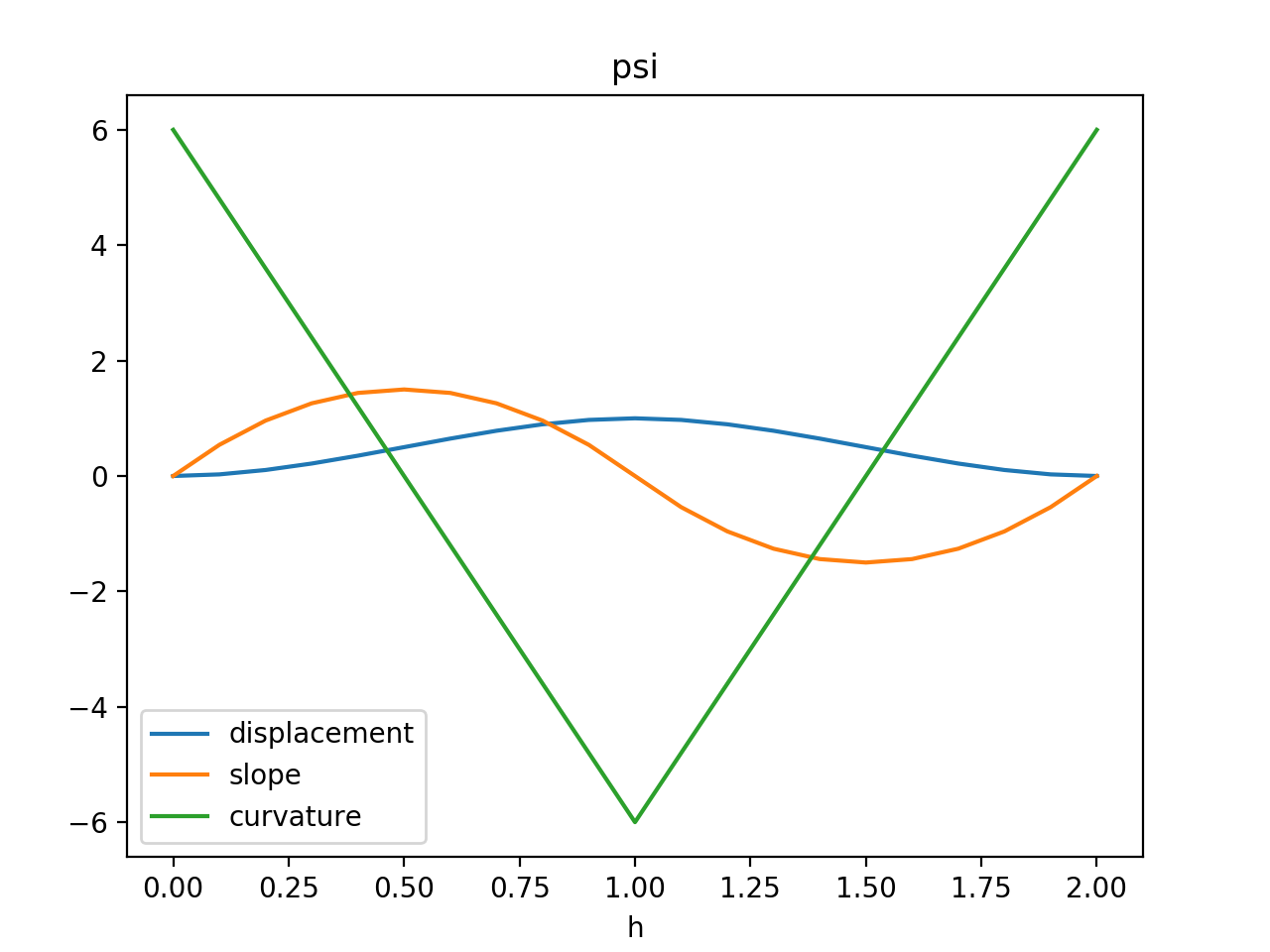
$\begin{aligned} p_1(x) &= 1 - \frac{3 x^{2}}{h^{2}} + \frac{2 x^{3}}{h^{3}} \\ p_2(x) &= x - \frac{2 x^{2}}{h} + \frac{x^{3}}{h^{2}} \\ p_3(x) &= \frac{3 x^{2}}{h^{2}} - \frac{2 x^{3}}{h^{3}} \\ p_4(x) &= - \frac{x^{2}}{h} + \frac{x^{3}}{h^{2}} \end{aligned}$

Now for $0 \leq i \leq n$ (I find zero-indexing convenient here so that the $i$ th basis function is centered at $ih$ ), define the basis functions

$\psi(x) = \begin{cases} p_3(x - (i - 1)h) &\text{ for } (i - 1)h < x < ih \\ p_1(x - ih) &\text{ for } ih \leq x < (i + 1)h \\ 0 &\text{ otherwise} \end{cases} \\ \zeta_i(x) = \begin{cases} p_4(x - (i - 1)h) &\text{ for } (i - 1)h < x < ih \\ p_2(x - ih) &\text{ for } ih \leq x < (i + 1)h \\ 0 &\text{ otherwise} \end{cases}$

Here’s what they look like. I’ve plotted their first and second derivatives as well.

psi

zeta

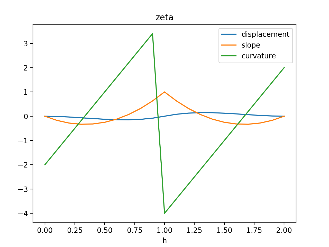
Both $\psi_i$ and $\zeta_i$ disappear at $(i-1)h$ and $(i+1)h$ (as do their derivatives). At $ih$ , $\psi_i$ has a value of one and a slope of zero, while $\zeta_i$ has a value of zero and a slope of one. Also note that the $0$ th and $n$ th basis functions must be defined slightly differently, since their domains must be restricted to the interval [0, 1]. I won’t write this out fully here, but I will take this into account going forward.

In the previous problem, we had to consider the different ways $\varphi_i$ and $\varphi_j$ could overlap. All integrals were zero except when $j = i$ or $j = i \pm 1$ , resulting in a tridiagonal matrix. The same concerns are at play here, but we also have to consider how our different basis functions interact. So, I’ll compute three matrices $\bold{A}^{\psi, \psi}$ , $\bold{A}^{\psi, \zeta}$ , and $\bold{A}^{\zeta, \zeta}$ as before. These can then be combined as blocks to generate $\bold{A}$ .

All three matrices are tridiagonal. $\bold{A}^{\psi, \psi}$ and $\bold{A}^{\zeta, \zeta}$ are symmetric. $\bold{A}^{\psi, \zeta}$ is not symmetric, since the left half of $\psi$ times the right half of $\zeta$ is not the same as the right half of $\psi$ times the left half of $\zeta$ . But we do have the symmetry that $\bold{A}^{\zeta, \psi}$ is the same as $(\bold{A}^{\psi, \zeta})^T$ . Also the interior diagonal elements of $\bold{A}^{\psi, \zeta}$ disappear, implying that $\psi$ and $\zeta$ are orthogonal. I’ll write out the matrices here for five vertices (including boundaries); for larger systems you’d just stretch them out along the diagonals. I wrote a Python script to compute all the entries, and print out the matrices in $\LaTeX$ .

$\bold{A}^{\psi, \psi} = \left[\begin{matrix}\frac{13 h}{35} & \frac{9 h}{70} & 0 & 0 & 0\\\frac{9 h}{70} & \frac{26 h}{35} & \frac{9 h}{70} & 0 & 0\\0 & \frac{9 h}{70} & \frac{26 h}{35} & \frac{9 h}{70} & 0\\0 & 0 & \frac{9 h}{70} & \frac{26 h}{35} & \frac{9 h}{70}\\0 & 0 & 0 & \frac{9 h}{70} & \frac{13 h}{35}\end{matrix}\right]$ $\bold{A}^{\zeta, \zeta} = \left[\begin{matrix}\frac{h^{3}}{105} & - \frac{h^{3}}{140} & 0 & 0 & 0\\- \frac{h^{3}}{140} & \frac{2 h^{3}}{105} & - \frac{h^{3}}{140} & 0 & 0\\0 & - \frac{h^{3}}{140} & \frac{2 h^{3}}{105} & - \frac{h^{3}}{140} & 0\\0 & 0 & - \frac{h^{3}}{140} & \frac{2 h^{3}}{105} & - \frac{h^{3}}{140}\\0 & 0 & 0 & - \frac{h^{3}}{140} & \frac{h^{3}}{105}\end{matrix}\right]$ $\bold{A}^{\psi, \zeta} = \left[\begin{matrix}\frac{11 h^{2}}{210} & - \frac{13 h^{2}}{420} & 0 & 0 & 0\\\frac{13 h^{2}}{420} & 0 & - \frac{13 h^{2}}{420} & 0 & 0\\0 & \frac{13 h^{2}}{420} & 0 & - \frac{13 h^{2}}{420} & 0\\0 & 0 & \frac{13 h^{2}}{420} & 0 & - \frac{13 h^{2}}{420}\\0 & 0 & 0 & \frac{13 h^{2}}{420} & - \frac{11 h^{2}}{210}\end{matrix}\right]$

I’ll assemble $\bold{A}$ as

$\bold{A} = \begin{bmatrix} \bold{A}^{\psi, \psi} & \bold{A}^{\psi, \zeta} \\ (\bold{A}^{\psi, \zeta})^T & \bold{A}^{\zeta, \zeta} \\ \end{bmatrix}$

Now we do the same for $\bold{B}$ . Note that $\bold{B}^{\zeta, \psi}$ is not $(\bold{B}^{\psi, \zeta})^T$ , since the boundary terms (from integrating by parts) differ.

$\bold{B}^{\psi, \psi} = \left[\begin{matrix}- \frac{6}{5 h} & \frac{6}{5 h} & 0 & 0 & 0\\\frac{6}{5 h} & - \frac{12}{5 h} & \frac{6}{5 h} & 0 & 0\\0 & \frac{6}{5 h} & - \frac{12}{5 h} & \frac{6}{5 h} & 0\\0 & 0 & \frac{6}{5 h} & - \frac{12}{5 h} & \frac{6}{5 h}\\0 & 0 & 0 & \frac{6}{5 h} & - \frac{6}{5 h}\end{matrix}\right]$ $\bold{B}^{\zeta, \zeta} = \left[\begin{matrix}- \frac{2 h}{15} & \frac{h}{30} & 0 & 0 & 0\\\frac{h}{30} & - \frac{4 h}{15} & \frac{h}{30} & 0 & 0\\0 & \frac{h}{30} & - \frac{4 h}{15} & \frac{h}{30} & 0\\0 & 0 & \frac{h}{30} & - \frac{4 h}{15} & \frac{h}{30}\\0 & 0 & 0 & \frac{h}{30} & - \frac{2 h}{15}\end{matrix}\right]$ $\bold{B}^{\psi, \zeta} = \left[\begin{matrix}- \frac{11}{10} & - \frac{1}{10} & 0 & 0 & 0\\\frac{1}{10} & 0 & - \frac{1}{10} & 0 & 0\\0 & \frac{1}{10} & 0 & - \frac{1}{10} & 0\\0 & 0 & \frac{1}{10} & 0 & - \frac{1}{10}\\0 & 0 & 0 & \frac{1}{10} & \frac{11}{10}\end{matrix}\right]$ $\bold{B}^{\zeta, \psi} = \left[\begin{matrix}- \frac{1}{10} & \frac{1}{10} & 0 & 0 & 0\\- \frac{1}{10} & 0 & \frac{1}{10} & 0 & 0\\0 & - \frac{1}{10} & 0 & \frac{1}{10} & 0\\0 & 0 & - \frac{1}{10} & 0 & \frac{1}{10}\\0 & 0 & 0 & - \frac{1}{10} & \frac{1}{10}\end{matrix}\right]$ $\bold{B} = \begin{bmatrix} \bold{B}^{\psi, \psi} & \bold{B}^{\psi, \zeta} \\ \bold{B}^{\zeta, \psi} & \bold{B}^{\zeta, \zeta} \\ \end{bmatrix}$

As a final note, I didn’t impose any boundary conditions on the system, so as currently stated the resulting system of ODEs is under-determined. To fix the boundaries at zero, one could remove $\psi_0$ and $\psi_n$ from the set of basis functions.

2

Model the bending of a beam (equation 9.29) under an applied load. Use Hermite polynomial interpolation, and boundary conditions fixing the displacement and slope at one end, and applying a force at the other end.

I answer this problem using two different sets of basis functions. The first technique uses cubic Hermite interpolation, and is implemented here. The second uses hat functions for the second derivative, integrating these to find the slopes and displacements. It is implemented here.

Cubic Hermite Interpolation

The potential energy of the beam is

$V = \int_0^L \left( \frac{1}{2} E I \left( \frac{d^2 u(x)}{dx^2} \right)^2 - u(x) f(x) \right) dx$

Our goal is to find a function $u(x)$ that makes $V$ stationary. We assume a solution of the form

$u(x) = \sum_{i=1}^n a_i \varphi_i(x)$

where the $a_i$ are unknown coefficients and $\varphi_i$ are a set of local basis functions.

Plugging this in,

$V = \int_0^L \left( \frac{1}{2} E I \left( \sum_{j=1}^n a_j \frac{d^2 \varphi_j(x)}{dx^2} \right)^2 - \left( \sum_{i=j}^n a_j \varphi_j(x) \right) f(x) \right) dx$

$\begin{aligned} \frac{\partial V}{\partial a_i} &= \int_0^L \left( E I \left( \sum_{j=1}^n a_j \frac{d^2 \varphi_j(x)}{dx^2} \right) \frac{d^2 \varphi_i(x)}{dx^2} - \varphi_i(x) f(x) \right) dx \\ &= \sum_{j=1}^n a_j E I \int_0^L \frac{d^2 \varphi_j(x)}{dx^2} \frac{d^2 \varphi_i(x)}{dx^2} dx - \int_0^L \varphi_i(x) f(x) dx \\ \end{aligned}$

We want all these partial derivatives to be zero. We can write the resulting system of equations as

$\bold{A} \overrightharpoon{a} = \overrightharpoon{b}$

where

$\begin{aligned} \bold{A}_{i,j} &= E I \int_0^L \frac{d^2 \varphi_i(x)}{dx^2} \frac{d^2 \varphi_j(x)}{dx^2} dx \\ b_i &= - \int_0^L \varphi_i(x) f(x) dx \end{aligned}$

I’ll use the basis functions $\psi$ and $\zeta$ as defined in the previous problem. If we use five nodes, the full blocks of $\bold{A}$ look like those below. Also as in the previous problem, $\bold{A}^{\zeta, \psi}$ is just $(\bold{A}^{\psi, \zeta})^T$ , so I won’t write it out.

$\bold{A}^{\psi, \psi} = \left[\begin{matrix}\frac{12}{h^{3}} & - \frac{12}{h^{3}} & 0 & 0 & 0\\- \frac{12}{h^{3}} & \frac{24}{h^{3}} & - \frac{12}{h^{3}} & 0 & 0\\0 & - \frac{12}{h^{3}} & \frac{24}{h^{3}} & - \frac{12}{h^{3}} & 0\\0 & 0 & - \frac{12}{h^{3}} & \frac{24}{h^{3}} & - \frac{12}{h^{3}}\\0 & 0 & 0 & - \frac{12}{h^{3}} & \frac{12}{h^{3}}\end{matrix}\right]$ $\bold{A}^{\zeta, \zeta} = \left[\begin{matrix}\frac{4}{h} & \frac{2}{h} & 0 & 0 & 0\\\frac{2}{h} & \frac{8}{h} & \frac{2}{h} & 0 & 0\\0 & \frac{2}{h} & \frac{8}{h} & \frac{2}{h} & 0\\0 & 0 & \frac{2}{h} & \frac{8}{h} & \frac{2}{h}\\0 & 0 & 0 & \frac{2}{h} & \frac{4}{h}\end{matrix}\right]$ $\bold{A}^{\psi, \zeta} = \left[\begin{matrix}\frac{6}{h^{2}} & \frac{6}{h^{2}} & 0 & 0 & 0\\- \frac{6}{h^{2}} & 0 & \frac{6}{h^{2}} & 0 & 0\\0 & - \frac{6}{h^{2}} & 0 & \frac{6}{h^{2}} & 0\\0 & 0 & - \frac{6}{h^{2}} & 0 & \frac{6}{h^{2}}\\0 & 0 & 0 & - \frac{6}{h^{2}} & - \frac{6}{h^{2}}\end{matrix}\right]$

But let’s think about our boundary conditions. Fixing the position and slope on one end of the beam means we’re fixing the coefficients of $\psi_0$ and $\zeta_0$ . So $\partial V / \partial \psi_0$ and $\partial V / \partial \zeta_0$ are irrelevant, and shouldn’t contribute any equations to our system. As such we basically need to chop the first row off these matrices (or at least $\bold{A}^{\psi, \psi}$ and $\bold{A}^{\zeta, \zeta}$ ). However if we do literally that, then we won’t have a square system anymore. So to keep our solver happy we’ll want to replace the missing rows with trivial equations $a_0 = a_0$ . This means zeroing out the whole row and adding a single one in the right place. (And when we get there, we’ll set $b_0$ to be the desired displacement or slope.) This breaks the symmetry of $\bold{A}^{\psi, \zeta}$ and $\bold{A}^{\zeta, \psi}$ , so we’ll want to compute each separately now.

$\bold{A}^{\psi, \psi} = \left[\begin{matrix}1 & 0 & 0 & 0 & 0\\- \frac{12}{h^{3}} & \frac{24}{h^{3}} & - \frac{12}{h^{3}} & 0 & 0\\0 & - \frac{12}{h^{3}} & \frac{24}{h^{3}} & - \frac{12}{h^{3}} & 0\\0 & 0 & - \frac{12}{h^{3}} & \frac{24}{h^{3}} & - \frac{12}{h^{3}}\\0 & 0 & 0 & - \frac{12}{h^{3}} & \frac{12}{h^{3}}\end{matrix}\right]$ $\bold{A}^{\zeta, \zeta} = \left[\begin{matrix}1 & 0 & 0 & 0 & 0\\\frac{2}{h} & \frac{8}{h} & \frac{2}{h} & 0 & 0\\0 & \frac{2}{h} & \frac{8}{h} & \frac{2}{h} & 0\\0 & 0 & \frac{2}{h} & \frac{8}{h} & \frac{2}{h}\\0 & 0 & 0 & \frac{2}{h} & \frac{4}{h}\end{matrix}\right]$ $\bold{A}^{\psi, \zeta} = \left[\begin{matrix}0 & 0 & 0 & 0 & 0\\- \frac{6}{h^{2}} & 0 & \frac{6}{h^{2}} & 0 & 0\\0 & - \frac{6}{h^{2}} & 0 & \frac{6}{h^{2}} & 0\\0 & 0 & - \frac{6}{h^{2}} & 0 & \frac{6}{h^{2}}\\0 & 0 & 0 & - \frac{6}{h^{2}} & - \frac{6}{h^{2}}\end{matrix}\right]$ $\bold{A}^{\zeta, \psi} = \left[\begin{matrix}0 & 0 & 0 & 0 & 0\\\frac{6}{h^{2}} & 0 & - \frac{6}{h^{2}} & 0 & 0\\0 & \frac{6}{h^{2}} & 0 & - \frac{6}{h^{2}} & 0\\0 & 0 & \frac{6}{h^{2}} & 0 & - \frac{6}{h^{2}}\\0 & 0 & 0 & \frac{6}{h^{2}} & - \frac{6}{h^{2}}\end{matrix}\right]$

Finally we assemble $\bold{A}$ as

$\bold{A} = \begin{bmatrix} \bold{A}^{\psi, \psi} & \bold{A}^{\psi, \zeta} \\ \bold{A}^{\zeta, \psi} & \bold{A}^{\zeta, \zeta} \\ \end{bmatrix}$

To compute $b_i$ , we need to choose a force distribution. I’ll apply a constant force $F$ to a fixed number of nodes near the end of the beam (the first and last only overlap the force region for half their basis functions). So

$b_i = - F \int_{0}^L \varphi_i(x) dx$

and is zero for all nodes not experiencing the force. Continuing with a 5 node demo system, I decided to apply the force to the last three nodes, and computed the following vectors.

$\begin{aligned} b^\psi &= \left[ 0, \ 0, \ \frac{F h}{2}, \ F h, \ \frac{F h}{2}\right] \\ b^\zeta &= \left[ 0, \ 0, \ \frac{F h^{2}}{12}, \ 0, \ - \frac{F h^{2}}{12}\right] \end{aligned}$

However we need to alter the first entries of these vectors to specify the boundary conditions. I’ll assume a displacement of zero, and a slope of 1/2.

$\begin{aligned} b^\psi &= \left[ 0, \ 0, \ \frac{F h}{2}, \ F h, \ \frac{F h}{2}\right] \\ b^\zeta &= \left[ 0.5, \ 0, \ \frac{F h^{2}}{12}, \ 0, \ - \frac{F h^{2}}{12}\right] \end{aligned}$

Finally, setting $E I = 1$ and $F = -10$ , and using numpy’s np.linalg.solve, I obtain a solution.

psi

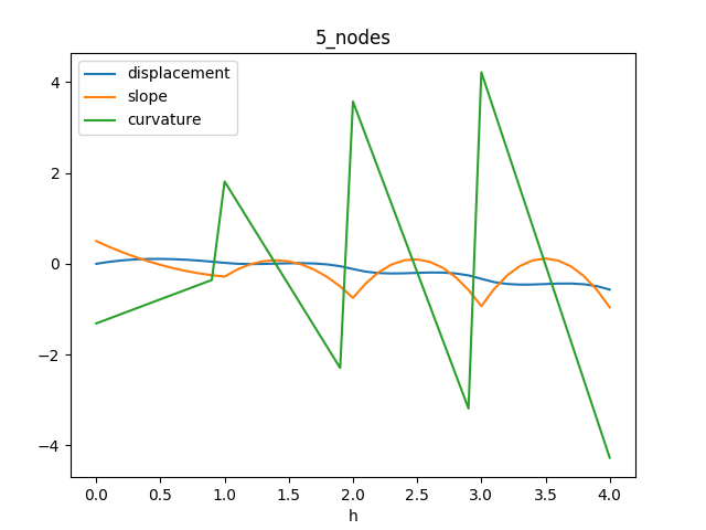
It’s unexpectedly wobbly. One way to get rid of this is to use only two nodes. But this kinda defeats the purpose of FEM.

psi

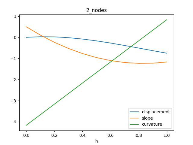
We should get a better solution with more elements, which is clearly not the case.

psi

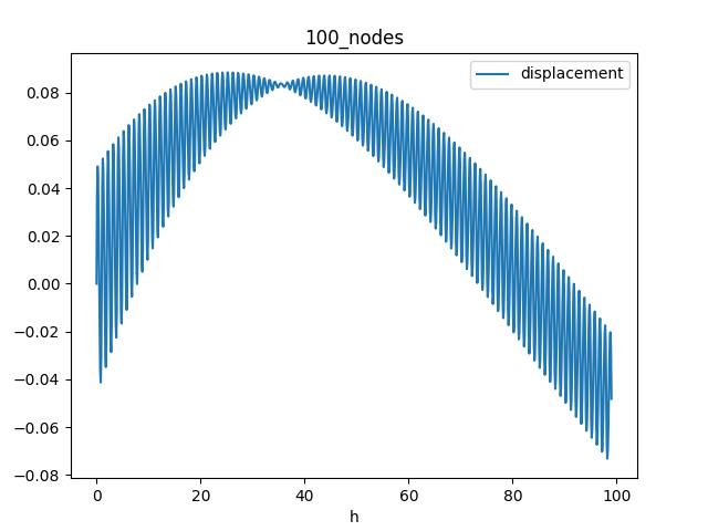
I might have a bug in here somewhere, but regardless I’m unhappy with these basis functions. $\zeta$ has a massive discontinuity in its second derivative, which is exactly what matters for the potential energy of the beam. So let’s try something different.

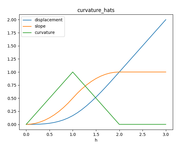
Hat Functions for the Second Derivative

In particular, since the second derivative is what’s most important, let’s model it directly.

$\frac{d^2 u(x)}{dx^2} = \sum_{i=1}^n a_i \varphi_i(x)$

We can find $u(x)$ by integrating. This produces an expression that’s no longer a sum of local basis functions, but that doesn’t matter for this problem.

$\begin{aligned} \frac{d u(x)}{dx} &= \sum_{i=1}^n a_i \int_0^x \varphi_i(x') dx' + s_0 \\ u(x) &= \sum_{i=1}^n a_i \int_0^x \int_0^{x'} \varphi_i(x'') dx'' dx' + s_0 x + u_0 \\ \end{aligned}$

Here $s_0$ is a constant of integration that determines the slope at $x = 0$ , and $u_0$ is a constant of integration that determines the displacement at $x = 0$ . The problem is invariant under translation up and down, so without loss of generality I’ll assume $u_0 = 0$ . (If we want to change this later, we just need to add the new $u_0$ to all the displacements we calculate for $u_0 = 0$ .) Here are what these basis functions look like.

psi

Side note: another way to develop a suitable set of basis functions would be to use 6th order Hermite interpolation. Then we could produce six shape functions, assembled into three basis functions. The extra degrees of freedom would allow us to ensure continuity for the second derivative, and add another basis function which would control the second derivative at a node. These basis functions would still be local.

Anyway, plugging in our nonlocal basis expansion yields

$\begin{aligned} V = &\int_0^L \frac{1}{2} E I \left( \sum_{j=1}^n a_j \varphi_j(x) \right)^2 dx \\ &-\int_0^L \left( \sum_{j=1}^n a_j \int_0^x \int_0^{x'} \varphi_j(x'') dx'' dx' + s_0 x \right) f(x) dx \end{aligned}$

$\begin{aligned} \frac{\partial V}{\partial a_i} = &\int_0^L E I \left( \sum_{j=1}^n a_j \varphi_j(x) \right) \varphi_i(x) dx \\ &-\int_0^L \left( \int_0^x \int_0^{x'} \varphi_i(x'') dx'' dx' + s_0 x \right) f(x) dx \\ = &\sum_{j=1}^n a_j E I \int_0^L \varphi_j(x) \varphi_i(x) dx \\ &-\int_0^L \left( \int_0^x \int_0^{x'} \varphi_i(x'') dx'' dx' \right) f(x) dx \\ &-s_0 \int_0^L x f(x) dx \\ \end{aligned}$

These define our new $\bold{A}$ and $\overrightharpoon{b}$ . Actually calculating them is very similar to with the previous basis functions, so I’ll only go over the differences. We’re back to using a single basis function, so $\bold{A}^{\varphi, \varphi}$ is the only $\bold{A}$ in town. It ends up symmetric and tridiagonal. Computing $\overrightharpoon{b}$ requires a good amount of integration so it was handy to use SymPy.

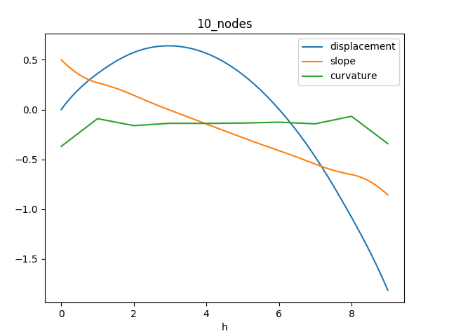
The results are much better.

psi

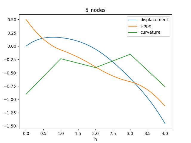
And now adding more nodes doesn’t make things worse.

psi