This week’s questions are all about exploring various optimization algorithms, so I won’t write them here specifically. This page summarizes my results. For notes on derivation and implementation, see here. Code is here.
I implemented Nelder-Mead, naive gradient descent (always step a constant factor times the gradient), and conjugate gradient descent. For the latter I initially used a golden section line search, but replaced it with Brent’s method. I still want to update it to use Brent’s method with derivatives. I also played around with the reference CMA-ES implementation for comparison.
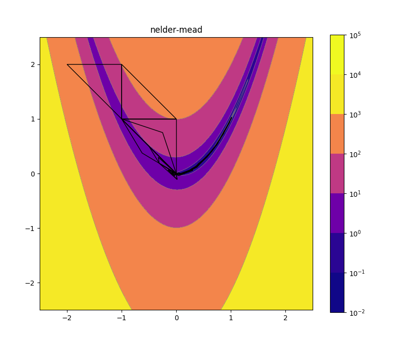
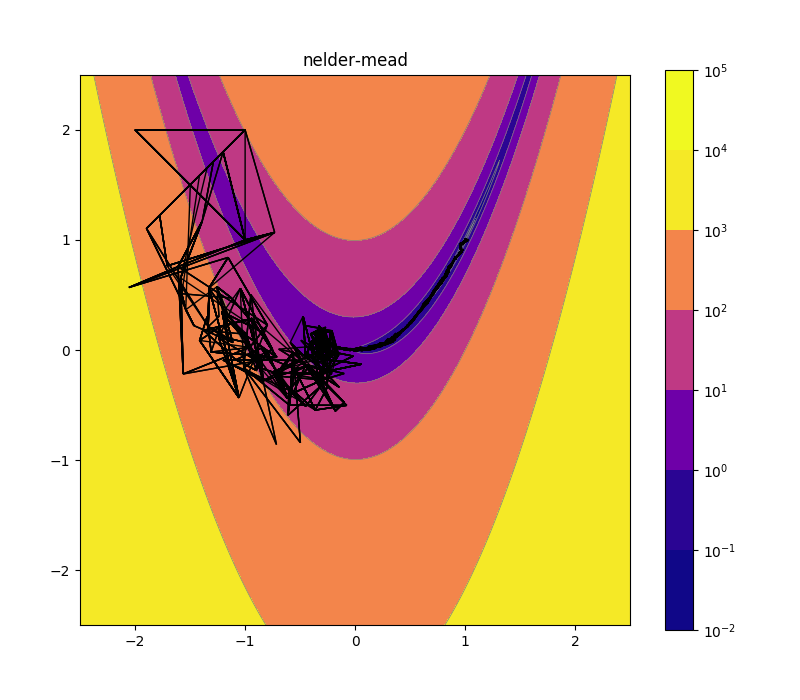
Nelder-Mead 2d
Nelder-Mead 10d
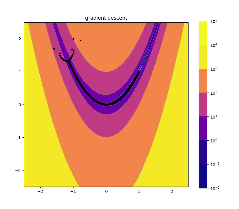
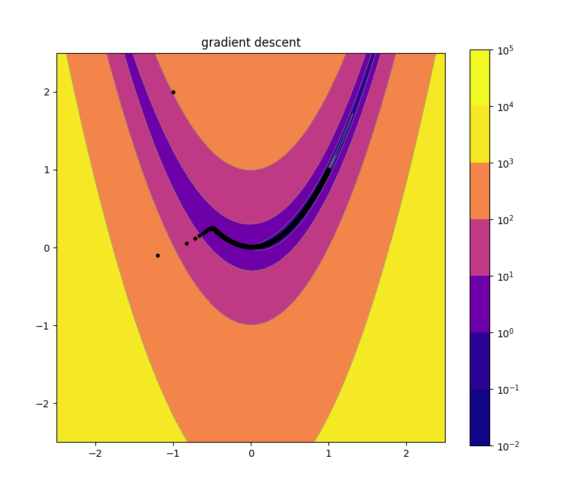
Naive Gradient Descent 2d
Naive Gradient Descent 10d
Conjugate Gradient Descent 2d

Conjugate Gradient Descent 10d

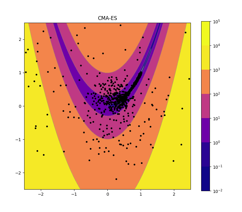
CMA-ES 2d

CMA-ES 10d
I haven’t made a pretty chart for this yet since I’m still playing around with the parameters (to make it as fair a fight as possible). But initial results suggest that on the multi-dimensional Rosenbrock function, conjugate gradient descent is a clear winner in scaling, at least through one thousand dimensions.
Here are some raw numbers. Nelder Mead and CMA-ES are asked to reach a tolerance of 1e-8, while the gradient descent methods are asked to find points where the gradient norm is less than 1e-8. These are the number of evaluations required to reach those goals, capped at 1e6.
Dim 2
nm:  193
gd:  28527
cgd: 1021
cma: 870

Dim 4
nm:  562
gd:  35724
cgd: 9448
cma: 2760

Dim 8
nm:  1591
gd:  45049
cgd: 5987
cma: 5790

Dim 16
nm:  27440
gd:  124637
cgd: 13083
cma: 14292

Dim 32
nm:  78969
gd:  200567
cgd: 13898
cma: 57876

Dim 64
nm:  561195
gd:  455578
cgd: 15194
cma: 211616

Dim 128
nm:  1000001
gd:  564451
cgd: 19565
cma: 953694

Dim 256
nm:  1000001
gd:  782196
cgd: 28110
cma: 1000000

Dim 512
nm:  1000001
gd:  1000000
cgd: 46918
cma: 1000000

Dim 1024
nm:  1000001
gd:  1000000
cgd: 10055
cma: 1000000
As a final note, all the algorithms except CMA-ES spent the majority of their time evaluating the function. But CMA-ES imposes large computational costs of its own, since it essentially has to invert a covariance matrix (or at least solve an eigenvalue problem).