I went rogue this week and did a deep dive on compressed sensing. So here’s the compressed sensing problem, followed by an exploration of compressed sensing CT reconstruction.
My code for all sections of this problem is here. All the sampling and gradient descent is done in C++ using Eigen for vector and matrix operations. I use Python and matplotlib to generate the plots.
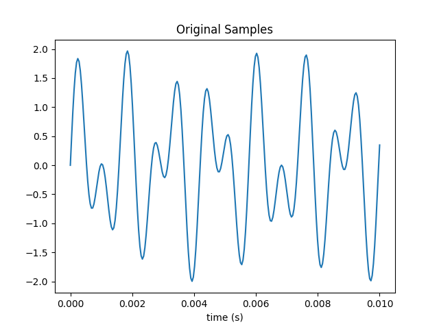
Generate and plot a periodically sampled time series {} of N points for the sum of two sine waves at 697 and 1209 Hz, which is the DTMF tone for the number 1 key.
Here’s a plot of 250 samples taken over one tenth of a second.
Calculate and plot the Discrete Cosine Transform (DCT) coefficients {} for these data, defined by their multiplication by the matrix , where
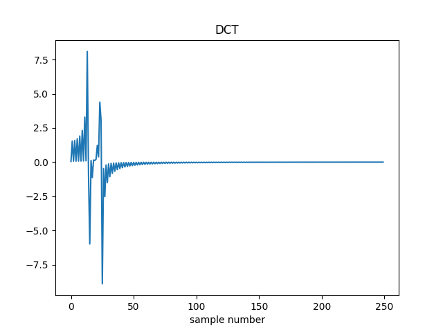
Plot the inverse transform of the {} by multiplying them by the inverse of the DCT matrix (which is equal to its transpose) and verify that it matches the time series.
The original samples are recovered.

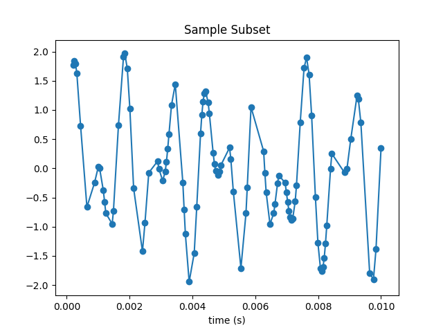
Randomly sample and plot a subset of M points {} of the {}; you’ll later investigate the dependence on the sample size.
Here I’ve selected 100 samples from the original 250. The plot is recognizable but very distorted.
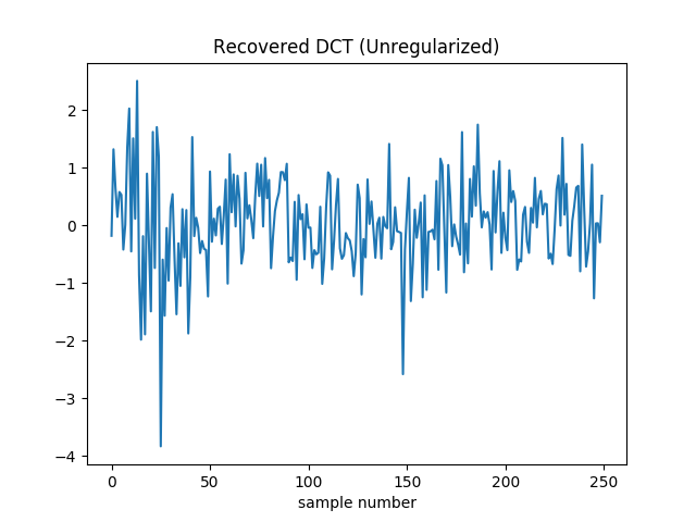
Starting with a random guess for the DCT coefficients {}, use gradient descent to minimize the error at the sample points
and plot the resulting estimated coefficients.
Gradient descent very quickly drives the loss function to zero. However it’s not reconstructing the true DCT coefficients.
To make sure I don’t have a bug in my code, I plotted the samples we get by performing the inverse DCT on the estimated coefficients.
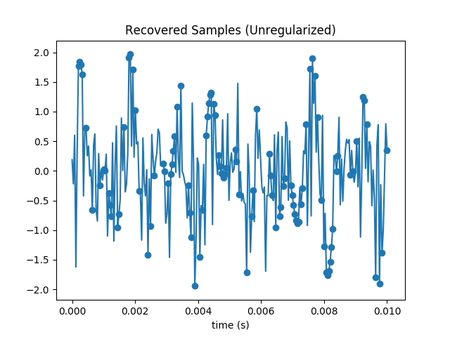
Sure enough all samples in the subset are matched exactly. But the others are way off the mark. We’ve added a lot of high frequency content, and are obviously overfitting.
The preceding minimization is under-constrained; it becomes well-posed if a norm of the DCT coefficients is minimized subject to a constraint of agreeing with the sampled points. One of the simplest (but not best [Gershenfeld, 1999]) ways to do this is by adding a penalty term to the minimization. Repeat the gradient descent minimization using the L2 norm:
and plot the resulting estimated coefficients.
With L2 regularization, we remove some of the high frequency content. This makes the real peaks a little more prominent.
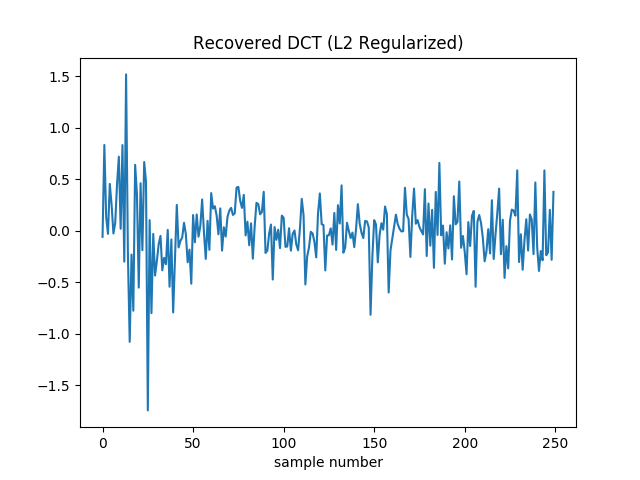
However it comes at a cost: gradient descent no longer drive the loss to zero. As such the loss itself isn’t a good termination condition. In its place I terminate when the squared norm of the gradient is less than . The final loss for the coefficients in the plot above is around 50.
You can easily see that the loss is nonzero from the reconstructed samples.
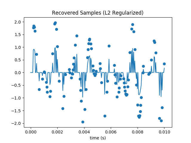
Repeat the gradient descent minimization using the L1 norm:
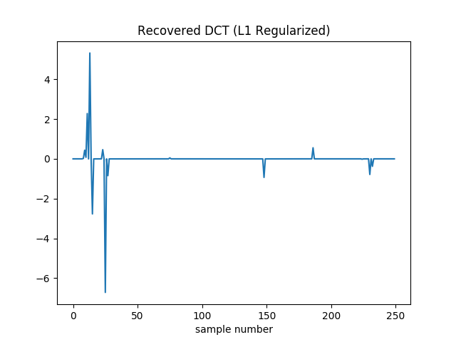
Plot the resulting estimated coefficients, compare to the L2 norm estimate, and compare the dependence of the results on M to the Nyquist sampling limit of twice the highest frequency.
With L1 regularization the DCT coefficients are recovered pretty well. There is no added high frequency noise.
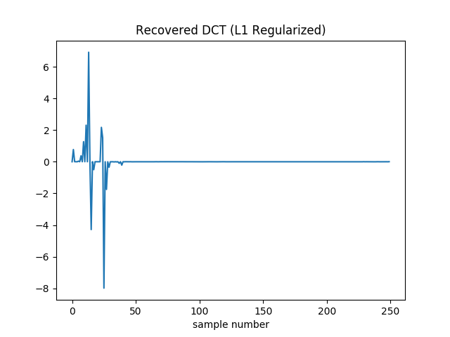
It still can’t drive the loss to zero. Additionally it’s hard to drive the squared norm of the gradient to zero, since the gradient of the absolute values shows up as 1 or -1. (Though to help prevent oscillation I actually drop this contribution if the absolute value of the coefficient in question is less than .) So here I terminate when the relative change in the loss falls below . I also decay the learning rate during optimization. It starts at 0.1 and is multiplied by 0.99 every 64 iterations.
The final loss is around 40, so better than we found with L2 regularization. However it did take longer to converge: this version stopped after 21,060 iterations, as opposed to 44 (for L2) or 42 (for unregularized). If I stop it after 50 samples it’s a bit worse than the L2 version (loss of 55 instead of 50). It’s not until roughly 2500 iterations that it’s unequivocally pulled ahead. I played with learning rates and decay schedules a bit, but there might be more room for improvement.
The recovered samples are also much more visually recognizable. The amplitude of our waveform seems overall a bit diminished, but unlike our previous attempts it looks similar to the original.
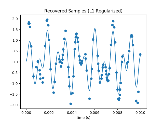
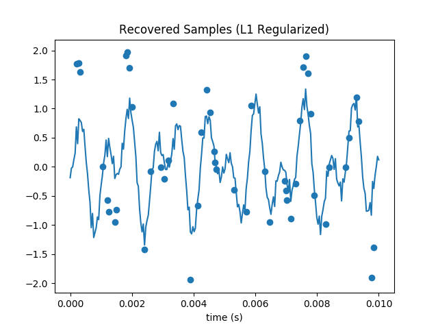
This technique can recover the signal substantially below the Nyquist limit. The highest frequency signal is 1209 Hz, so with traditional techniques we’d have to sample at 2418 Hz or faster to avoid artifacts. Since I’m only plotting over one hundreth of a second, I thus need at least 242 samples. So my original 250 is (not coicidentally) near here. But even with a subset of only 50 samples, the L1 regularized gradient descent does an admirable job at recovering the DCT coefficients and samples:
Code lives here.
Last year my final project for The Physics of Information Technology dealt with reconstruction of CT images. I explored the classic techniques like filtered back projection, then started but didn’t finish a compressed sensing based approach. Recently I revisited this and it finally works.
For basic context, a computed tomography machine takes xray images of an object from a number of different angles. No one of these gives an internal slice of the object; they’re all projections. But using the right mathematical techniques, it’s possible to infer the interior structure of the object.
Compressed sensing reconstruction, in broad strokes, works just like the DCT problem above, except instead of using a DCT, one simulates taking the xray images. Let’s work through the reconstruction of a horizontal 2D slice. Each xray projection gives a 1D image, i.e. a row of pixel values. Traditionally these are all stacked into a single image like this.
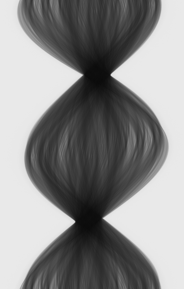
This is called a sinogram. Each row of pixels is a projection. Moving from top to bottom corresponds to the rotation of the object. This particular sinogram was generated by CBA’s CT machine. It’s a scan of a piece of coral. This is the raw data that we want to match; it’s the equivalent of the DCT coefficients from the previous problem.
The transform we need to implement then, is from a 2D image to its projections. That is, given an image where each pixel represents the transmissivity of that region of space for xrays, we need to generate the resulting sinogram. Essentially this boils down to an elementary ray tracing algorithm.
Once we have this, we can run an optimization algorithm that tunes the pixel values to produce the correct sinogram. My implementation computes the loss gradient as well as the loss, so I can use conjugate gradient descent (as implemented for the problem set before this one). A total variation (TV) regularization term is applied, essentially summing the absolute value of the gradient of the transmissivity at each pixel. This damps out noise, and encourages blocks of homogenous density as are common in biological and mechanical samples.
On to the results. Using all the data, here’s a reconstructed slice of coral.
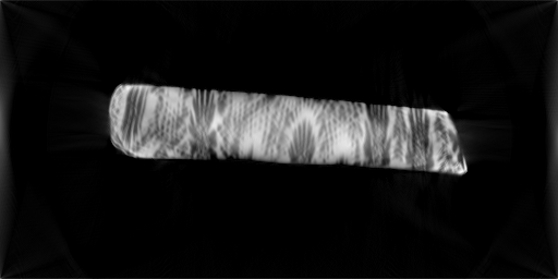
Surprisingly, so far I haven’t found much of a difference with and without the TV term. Here I use only 2% of the projections. With TV I get this:

And without:
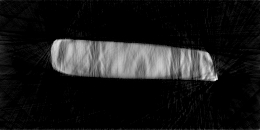
Regardless, the construction quality is much poorer with the limited data.