The Lattice-Boltzmann for Fluid Dynamics
Summary
In this project I implement the Lattice Boltzmann (LB) method for Fluid Dynamics to gain understanding how unsteady flow behavior arises in a cylinder cross-flow. The LBM method is implented efficiently using NumPy in Python. Numerical experiments are pefromed at different Reynolds numbers, namely the ratio of viscous to inertial forces, starting from Re=5 to Re = 500. Unsteady fluid behavior starts to arise for Re>53 and typically at Re>90 we get a fully developed Karman vortex street, whose frequency and amplitude increases as the Re increases. These simulations can be used only as a qualitative and semi-quantitative tool for studying this phenomenon.
Report
The Boltzmann Distribution on a Lattice
Suppose that the fluid is an ideal gas, and suppose for now that it has a macroscopic velocity $\vec{u}$ and is in thermal equilibrium at temperature $T$.
Then, the molecules will have thermal velocities $\vec{v}$ that are distributed according to the Boltzmann distribution of statistical mechanics.
For a two-dimensional gas, this distribution is:
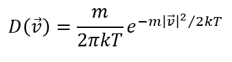
where, where $m$ is the mass of each molecule and $k$ is Boltzmann's constant. This is the function which, when integrated over any range of $v_x$ and $v_y$, gives the probability that a particular molecule will have a velocity in that range.
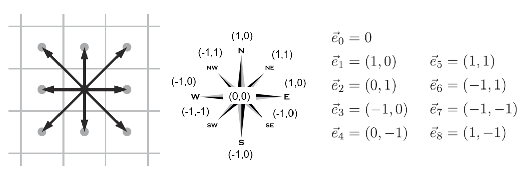
In the lattice-Boltzmann approach, we discretize both space and time so that only certain discrete velocity vectors are allowed. In this project, we will use the so-called D2Q9 lattice in which there are two dimensions and just nine allowed displacement vectors, as shown below:
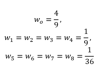
Our task, now, is to attach probabilities to these nine velocity vectors, to model the continuous Boltzmann distribution as accurately as possible. For a fuid at rest ($\vec{u} = 0$), the previous equation gives the most and least probable velocities with following probabilities or weights $w_i$ for each of the nine directions:
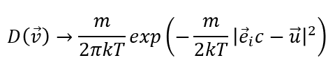
The total velocity of any molecule is $\vec{u}$ plus the thermal velocity $\vec{v}$, and we will still constrain this total velocity to be one of our nine lattice velocities:

The Boltzmann distribution for thermal velocities is unaffected by $\vec{u}$, so we can plug this difference into the very first equation to obtain a new set of probabilities:
A little bit of math...

The Lattice-Boltzmann Algorithm
In a lattice-Boltzmann simulation, the fundamental dynamical variables are the nine different number densities, of molecules moving at the nine allowed velocities, at each lattice site.
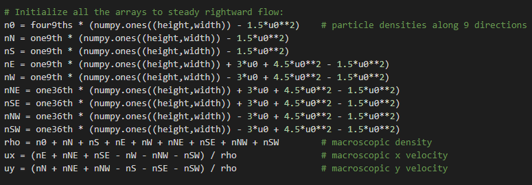
At any given time, at a given lattice site, these nine densities can have any positive values. From these values you can then compute the total density, $\rho$, as well as the x and y components of the average (that is, macroscopic) velocity, uxand uy. And from these three macroscopic variables, you can compute what the nine densities would be if the molecules at this site were in thermal equilibrium:

The most obvious next step would then be to set all the nine densities equal to these equilibrium values; doing so would mimic the process of collisions among the molecules, which brings them closer to thermal equilibrium. But the time scale for reaching equilibrium needn't be identical to the time step of the simulation. So a more general procedure is to change the value of each ni toward its equilibrium value by a variable fraction:
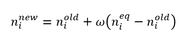
Here $\omega$ is a unitless number that can vary between about 0 and 2.
- smaller $\omega$ $\rightarrow$ slower collisions to reach equilibrium - highlyviscous fluid
- larger $\omega$ $\rightarrow$ faster collisions
The LB algorithm consists of the following steps:
- Discretization of the 2-D space with a square lattice.
- 9 discplacements and velocities are allowed at each node.
- Simulation variables $n_i$ are the 9 densities, at each lattice site, of molecules with the 9 allowed velocities.
- Using the above variables the total density $\rho$ and the macroscopic flow velocity $\vec{u}$ are computed as:
$\rho = \sum{n_i}$ | $u_x = \frac{(n_1 + n_5 + n_8)-(n_3 + n_6 + n_7)}{\rho}$ | $u_y = \frac{(n_2 + n_5 + n_6)-(n_4 + n_7 + n_8)}{\rho} $
- Thermal velocities ($\vec{u}$) are modeled based on the discretization of the Boltzmann distribution. Weights are determined by equating moments,
up to 4th order, of the continuous and discrete distributions, as previously explained.
- Total (discretized velocities) velocity is flow velocity plus thermal velocity. After pluging into the Boltzmann distribution and expand to 2nd order
in $\vec{u}$, equilibrium densities can be obtained.
- During each time step, molecules within each lattice cell collide and relax toward these equilibrium values, by an amount that depends on the relaxation time
$\tau$ (which increases with increasing viscosity).
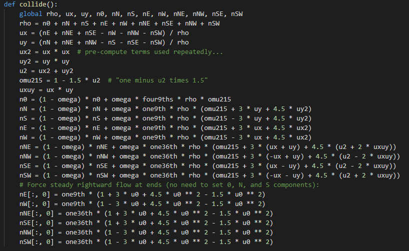
- The algorithm is simply to alternate these collisions with a streaming step during which the molecules move into adjacent cells according to their discretized velocities and when molecules hit a barrier they bounce back.
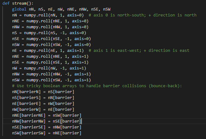
On boundaries we apply periodicity. The complication here is that you have to handle separately populations which are on our domain boundary, and which are streamed out of the domain. You have to do something with them. What I chose to do in this code, is to take them, stream them out of the domain and re-inject them into the domain in the opposite direction. In this way, we have periodic boundary conditions, everything which leaves things to domain on the left, enters on the right. If it leaves on the right, it enters on the left. If it leaves on the top, it enters on the bottom, and vice versa.We call this periodic boundary condition because the system behaves as if it was periodically repeated an infinite amount of times in the direction in which it is periodic. NumPy offers a function which is called roll which will shift a matrix periodically in one of the space directions. To do the streaming step, I call the roll function twice, once to shift it by the right amount of cells in x direction and once to shift it by the right amount of cells in y direction. The number of cells by which it is shifted is either 1, or -1, and it's given by the value of the Lattice velocity indicating space direction. So the NumPy array-based code for the streaming step is nothing else than a loop over nine space directions, a double call to the roll function of the outgoing populations. As a parameter, axis 0 for the x direction, axis 1 for y direction, and the amount of shifts given by Lattice velocities. And we copy the results back into the incoming populations to have them ready for the next collision step.