Week 8

Search

Link to completed assignment

Problem 15.1

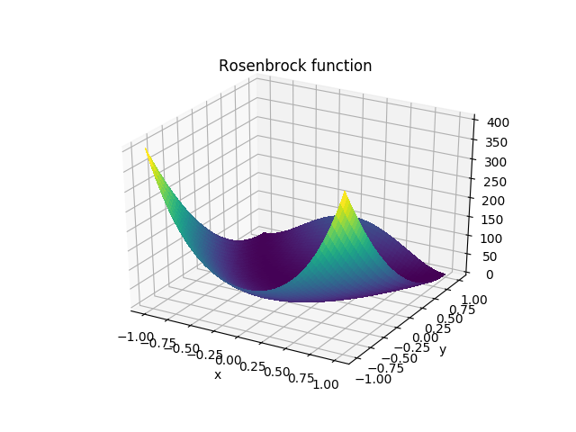
(a) The first thing we need to do is plot the Rosenbrock function, $$f = (1-x)^2 + 100(y-x^2)^2$$


      import matplotlib
      matplotlib.use('Agg')
      import matplotlib.pyplot as plt
      from mpl_toolkits import mplot3d
      import numpy as np

      def rosenbrock(x, y):
          return ((1 - x)**2 + 100*(y - x**2)**2)

      x = np.linspace(-1,1,1000)
      y = np.linspace(-1,1,1000)

      X, Y = np.meshgrid(x, y)
      F = rosenbrock(X, Y)

      fig = plt.figure()
      ax = plt.axes(projection='3d')
      ax.set_xlabel('x')
      ax.set_ylabel('y')
      ax.set_title('Rosenbrock function')
      surf = ax.plot_surface(X, Y, F, cmap='viridis', linewidth=0, antialiased=False)
      plt.savefig('./plots/search.png')

(b) Now, we will use the downhill simplex method to search for the function's minimum, starting from x = y = -1. Using the scipy.optimize.minimize function, we are able to determine the number of algorithm iterations and function evaluations used, as well as the final values of where the minimum is located.


      import numpy as np
      from scipy.optimize import minimize

      def rosenbrock(x):
        return ((1 - x[:-1])**2 + 100*(x[1:] - x[:-1]**2)**2)

      x0 = np.array([-1, -1])

      print(minimize(rosenbrock, x0, method='Nelder-Mead'))

Algorithm iterations	67
Function evaluations	125
Final minimum location	(0.99999886, 0.99999542)

(c) We will now repeat this process in 10D instead of 2D, using the following D-dimensional generalization of the Rosenbrock function: $$f = \sum_{i=1}^{D-1} (1-x_{i-1})^2 + 100(x_i - x_{i-1}^2)^2$$ Starting with all x_i at -1, we will again count the algorithm iterations and function evaluations.


      import numpy as np
      from scipy.optimize import minimize

      def rosenbrock(x):
        d = len(x)
        sum = 0
        for i in range(d):
          xi = x[i]
          xprev = x[i-1]
          new = (1-xprev)**2 + 100*(xi - xprev**2)**2
          sum = sum + new
        return sum

      x0 = np.array([-1, -1, -1, -1, -1, -1, -1, -1, -1, -1])

      print(minimize(rosenbrock, x0, method='Nelder-Mead'))

Algorithm iterations	1048
Function evaluations	1459
Final minimum location	(0.01023648, 0.01024337, 0.01023174, 0.01019699, 0.01016837, 0.01022307, 0.01023505, 0.0102289 , 0.01024435, 0.01018521)

(d) Now, we will repeat and compare the 2D and 10D Rosenbrock search with the conjugate gradient method.

(e) Now, we will repeat and compare the 2D and 10D Rosenbrock search with CMA-ES.

(f) Finally, we will explore how these algorithms perform in higher dimensions. We will specifically take a look at the D-dimensional generalization of the Rosenbrock function being evaluated by the Nelder-Mead method of various dimensions.


      import numpy as np
      from scipy.optimize import minimize

      Dim_analysis = [2, 3, 4, 5, 10, 12, 15]

      for D in Dim_analysis:

          def rosenbrock(x):
              d = len(x)
              sum = 0
              for i in range(d):
                  xi = x[i]
                  xprev = x[i-1]
                  new = (1-xprev)**2 + 100*(xi - xprev**2)**2
                  sum = sum + new
              return sum

          x0 = -1*np.ones(D)

          print(minimize(rosenbrock, x0, method='Nelder-Mead'))

Dimensions	2	3	4	5	10	12	15
Algorithm iterations	40	86	134	180	1048	1789	2341
Function evaluations	70	151	229	301	1459	2401*	3000*
*Maximum number of function evaluations was exceeded.