Function Architectures
Week 10
Link to completed assignment
Problem 14.1
Problem 14.1
To find the first five diagonal Pade approximants [1/1],...,[5/5] to the function ex, we start by taking the Taylor series expansion of the function: $$e^x = \sum_{n=0}^{\infty} \frac{x^n}{n!}$$ As in Eq. (14.3), we will compare that Taylor expansion to the general form: $$f(x) = \sum_{l=0}^{\infty} c_l x^l$$ Which will then make it fit nicely in the Pade approximant formula as in Eq. (14.4): $$\frac{\sum_{n=0}^N a_n x^n}{1 + \sum_{m=1}^M b_m x^m} = \sum_{l=0}^L c_l x^l$$ After a little more solving, we can get the following equations to help us solve for our a and b coefficients. First, Eq. (14.6) gives us a: $$a_n = c_n + \sum_{m=1}^N b_m c_{n-m} \quad (n=0,...,N)$$ Remember that $$c_n = \frac{1}{n!}$$ Which helps us figure out how to index the different coefficients arrays and matrices in the code. We also have b from Eq. (14.7): $$0 = c_l + \sum_{m=1}^M b_m c_{l-m} \quad (l=N+1,...,N+M)$$ We have to do a little bit of linear algebra to extract the b coefficients out of there, but it all works out. Once all that is taken care of, we can take the original fraction from the left-hand side of Eq. (14.4) to find out the value of the Pade approximation, plugging in x=1. We will also check to see how accurate the approximation is to the real value of e1 = 2.718281828459045.
      import math
      import numpy as np

      def pade_approx(N):
          b = solve_b_coef(N)
          a = solve_a_coef(N, b)
          num = a.dot(np.ones(N+1))
          den = 1 + b.dot(np.ones(N))
          val = num / den
          return val

      def solve_b_coef(N):
          C_lm = np.zeros((N, N))
          C_l = np.zeros(N)
          for i in range(N):
              C_l[i] = -1/math.factorial(N+1+i)
              for j in range(N):
                  C_lm[i][j] = 1/math.factorial(N+1+i-(1+j))
          B = np.linalg.pinv(C_lm).dot(C_l)
          return B

      def solve_a_coef(N, B):
          A = np.zeros(N+1)
          for i in range(N+1):
              A[i] += 1/math.factorial(i)
              for j in range(1, i+1):
                  A[i] += B[j-1]/math.factorial(i-j)
          return A

      e = 2.718281828459045
      start = 1
      stop = 5
      print()

      for N in range (start,stop+1):
          val = pade_approx(N)
          error = abs(val - e)

          print("Pade Approximant", N)
          print("Value:    ", val)
          print("Actual:   ", e)
          print("|Error|:  ", error)
          print()
The code above gives us the following results:
      Pade Approximant 1
      Value:     3.0
      Actual:    2.718281828459045
      |Error|:   0.2817181715409549

      Pade Approximant 2
      Value:     2.7142857142857144
      Actual:    2.718281828459045
      |Error|:   0.003996114173330678

      Pade Approximant 3
      Value:     2.71830985915493
      Actual:    2.718281828459045
      |Error|:   2.8030695884861956e-05

      Pade Approximant 4
      Value:     2.718281718281719
      Actual:    2.718281828459045
      |Error|:   1.1017732592932816e-07

      Pade Approximant 5
      Value:     2.7182818287356953
      Actual:    2.718281828459045
      |Error|:   2.7665025825740486e-10
We can see that the error improves greatly with the order of the Pade approximants. For the first five diagonal Pade approximants, the error improves by 2 or 3 orders of magnitude with each step.
Problem 14.2
We will be working with the following data set: $$x = {-10,\ -9,\ ...,\ 9,\ 10}$$ $$y = \begin{cases} 0, \ x \le 0 \\[2ex] 1, \ x \gt 0 \\[2ex] \end{cases}$$
      import matplotlib
      matplotlib.use('Agg')
      import matplotlib.pyplot as plt
      import numpy as np

      def data(x_min, x_max):
          x = np.arange(x_min, x_max + 1)
          n = len(x)
          y = np.zeros(n)
          for i in range(n):
              if (x[i] > 0):
                  y[i] = 1
          return x, y, n

      def plot_data(x, y):
          plt.clf()
          plt.plot(x, y, label='Data')
          plt.xlim(x[0] - 1, x[-1] + 1)
          plt.ylim(y[0] - 0.2, y[-1] + 0.2)

      x, y, n = data(-10, 10)
      plot_data(x, y)
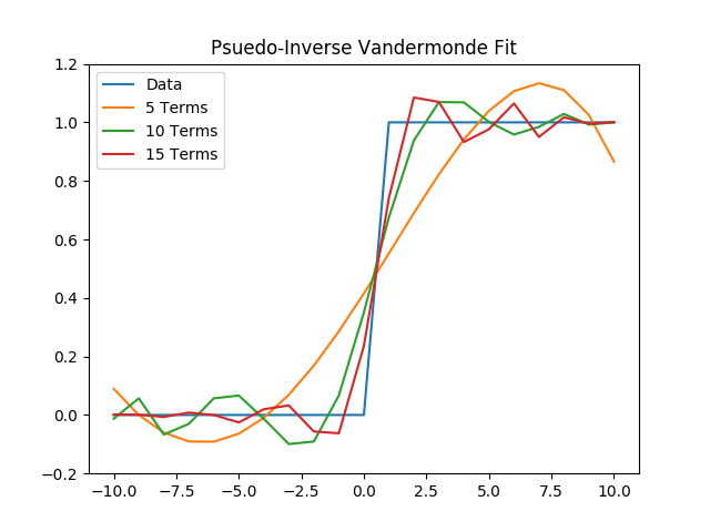
(a) First, we will fit the data with a polynomial with 5, 10, and 15 terms, using a psuedo-inverse of the Vandermonde matrix.
      def vandermonde(n, m, x, y):
          A = np.zeros((n, m))
          for i in range(n):
              for j in range(m):
                  A[i][j] = x[i]**j
          return np.linalg.pinv(A).dot(y)

      def vandermonde_fit(n, m, x, coef):
          y = np.zeros(n)
          for i in range(n):
              for j in range(m):
                  y[i] += coef[j]*x[i]**j
          return y

      terms = [5, 10, 15]

      for m in terms:
          coef = vandermonde(n, m, x, y)
          y_vand = vandermonde_fit(n, m, x, coef)
          plt.plot(x, y_vand, label=str(m) + ' Terms')

      plt.title("Psuedo-Inverse Vandermonde Fit")
      plt.legend()
      plt.savefig('./plots/function_architecture/vandermonde.png')
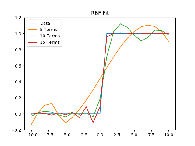
(b) Then, we will fit the data with 5, 10, and 15 r3 RBFs uniformly distributed between x = -10 and x = 10.
      def centers(m):
          c = np.zeros(m)
          for i in range(m):
              c[i] = (20)*(np.random.rand()-0.5)
          return c

      def rbf(n, m, x, y, c):
          A = np.zeros((n, m))
          for i in range(n):
              for j in range(m):
                  A[i][j] = np.abs(x[i]-c[j])**3
          return np.linalg.pinv(A).dot(y)

      def rbf_fit(n, m, x, c, coef):
          y = np.zeros(n)
          for i in range(n):
              for j in range(m):
                  y[i] += coef[j]*np.abs(x[i]-c[j])**3
          return y

      plot_data(x, y)

      for m in terms:
          c = centers(m)
          coef = rbf(n, m, x, y, c)
          y_rbf = rbf_fit(n, m, x, c, coef)
          plt.plot(x, y_rbf, label=str(m) + ' Terms')

      plt.title("RBF Fit")
      plt.legend()
      plt.savefig('./plots/function_architecture/rbf.png')
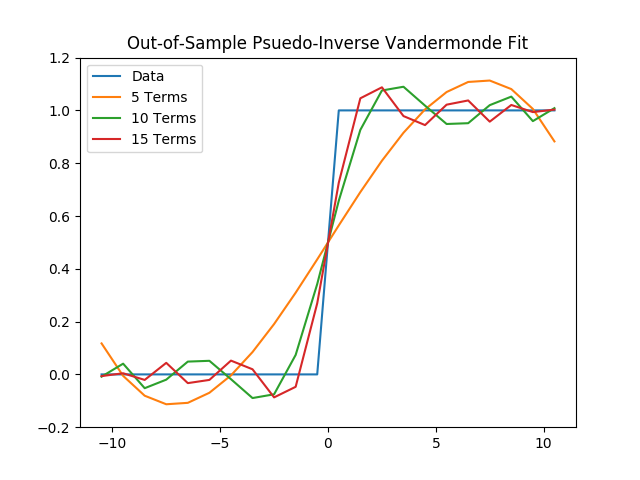
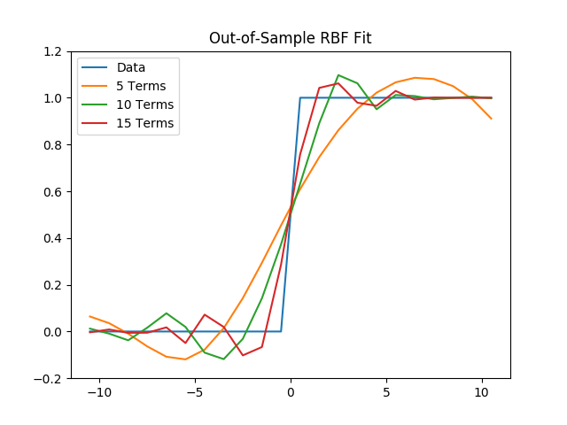
(c) Next, using the coefficients found for these six fits, we will evaluate the total out-of-sample error at $$x = {-10.5,\ -9.5,\ ...,\ 9.5,\ 10.5}.$$
      x_oos, y_oos, n_oos = data(-10.5, 10.5)
      plot_data(x_oos, y_oos)

      for m in terms:
          coef = vandermonde(n_oos, m, x_oos, y_oos)
          y_vand_oos = vandermonde_fit(n_oos, m, x_oos, coef)
          plt.plot(x_oos, y_vand_oos, label=str(m) + ' Terms')

      plt.title("Out-of-Sample Psuedo-Inverse Vandermonde Fit")
      plt.legend()
      plt.savefig('./plots/function_architecture/vandermonde_oos.png')

      plot_data(x_oos, y_oos)

      for m in terms:
          c = centers(m)
          coef = rbf(n_oos, m, x_oos, y_oos, c)
          y_rbf_oos = rbf_fit(n_oos, m, x_oos, c, coef)
          plt.plot(x_oos, y_rbf_oos, label=str(m) + ' Terms')

      plt.title("Out-of-Sample RBF Fit")
      plt.legend()
      plt.savefig('./plots/function_architecture/rbf_oos.png')
(d) Finally, using a 10th-order polynomial, we wil fit the data with the curvature regularizer in equation (14.53): $$I = \sum_{n=1}^N [y_n - f(x_n, a)]^2 + \lambda \int \bigl[ \frac{d^2 f}{dx^2} \bigr]^2$$ We will then plot the fits for λ = 0, 0.01, 0.1, 1.
Problem 14.3
We will train a neural network on the output from an order 4 maximal LFSR (see Problem 6.3) and learn to reproduce it. We will then analyze how the results depend on the network depth and architecture. First, the code to produce our data:
      import numpy as np

      def generate_data(n, x):
          input = []
          output = []
          for i in range(n):
              input.append(x)
              x_n = x[0] ^ x[3]
              output.append(x_n)
              x = [x_n, x[0], x[1], x[2]]
          return input, output

      seed = [1, 1, 1, 1]
      x_data, y_data = generate_data(16, seed)

      for i in range(len(x_data)):
          print("Input:", x_data[i], "Output:", y_data[i])
This gives us the following data. Note that this data set will repeat indefinitely depending on how many iterations the generate_data(n, x) function runs.
      Input: [1, 1, 1, 1] Output: 0
      Input: [0, 1, 1, 1] Output: 1
      Input: [1, 0, 1, 1] Output: 0
      Input: [0, 1, 0, 1] Output: 1
      Input: [1, 0, 1, 0] Output: 1
      Input: [1, 1, 0, 1] Output: 0
      Input: [0, 1, 1, 0] Output: 0
      Input: [0, 0, 1, 1] Output: 1
      Input: [1, 0, 0, 1] Output: 0
      Input: [0, 1, 0, 0] Output: 0
      Input: [0, 0, 1, 0] Output: 0
      Input: [0, 0, 0, 1] Output: 1
      Input: [1, 0, 0, 0] Output: 1
      Input: [1, 1, 0, 0] Output: 1
      Input: [1, 1, 1, 0] Output: 1
      Input: [1, 1, 1, 1] Output: 0
The following code is my attempt to use Tensorflow to write my own neural network to be trained from the data I generated (I would generate many more sets for the actual training data). It would then learn to predict and reproduce the output data from the true data. Unfortunately, I wasn't able to completely figure out how to get the code to run. I followed the following tutorial to set up this neural network: https://adventuresinmachinelearning.com/python-tensorflow-tutorial/
      import tensorflow.compat.v1 as tf
      import tensorflow_datasets as tfds
      tf.disable_v2_behavior()
      dataset = tfds.load(name="mnist", split=tfds.Split.TRAIN)

      from tensorflow.examples.tutorials.mnist import input_data
      mnist = input_data.read_data_sets("MNIST_data/", one_hot=True)

      learning_rate = 0.5
      epochs = 10
      batch_size = 100

      x = tf.placeholder(tf.float32, [None, 4])
      y = tf.placeholder(tf.float32, [None, 2])

      W1 = tf.Variable(tf.random_normal([4, 3], stddev=0.03), name='W1')
      b1 = tf.Variable(tf.random_normal([3]), name='b1')
      W2 = tf.Variable(tf.random_normal([3, 2], stddev=0.03), name='W2')
      b2 = tf.Variable(tf.random_normal([2]), name='b2')

      hidden_out = tf.add(tf.matmul(x, W1), b1)
      hidden_out = tf.nn.relu(hidden_out)

      y_ = tf.nn.softmax(tf.add(tf.matmul(hidden_out, W2), b2))

      y_clipped = tf.clip_by_value(y_, 1e-10, 0.9999999)
      cross_entropy = -tf.reduce_mean(tf.reduce_sum(y * tf.log(y_clipped) + (1 - y) * tf.log(1 - y_clipped), axis=1))

      optimiser = tf.train.GradientDescentOptimizer(learning_rate=learning_rate).minimize(cross_entropy)

      init_op = tf.global_variables_initializer()

      correct_prediction = tf.equal(tf.argmax(y, 1), tf.argmax(y_, 1))
      accuracy = tf.reduce_mean(tf.cast(correct_prediction, tf.float32))

      with tf.Session() as sess:
         sess.run(init_op)
         total_batch = int(len(mnist.train.labels) / batch_size)
         for epoch in range(epochs):
              avg_cost = 0
              for i in range(total_batch):
                  batch_x, batch_y = mnist.train.next_batch(batch_size=batch_size)
                  _, c = sess.run([optimiser, cross_entropy], feed_dict={x: batch_x, y: batch_y})
                  avg_cost += c / total_batch
              print("Epoch:", (epoch + 1), "cost =", "{:.3f}".format(avg_cost))
         print(sess.run(accuracy, feed_dict={x: mnist.test.images, y: mnist.test.labels}))