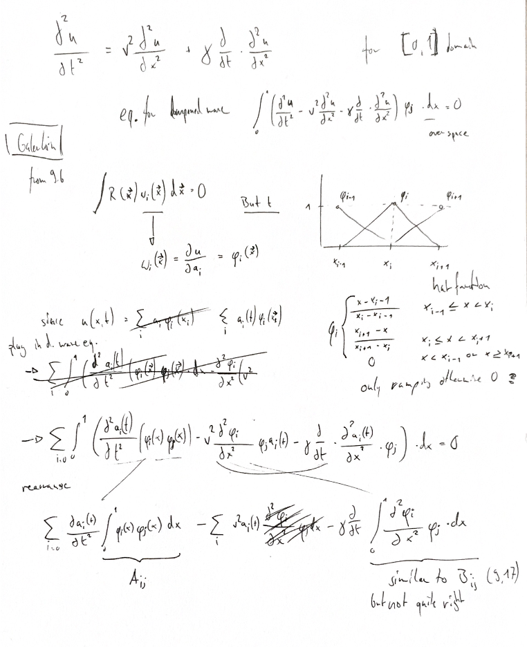
Problem 9.1

a) Use the Galerkin method to find an approximating system of differential equations.

Failed to rearrange. Have to ceom back to that.

b) Evaluate the matrix coefficients for linear hat basis functions, using elements with a fixed size of h.

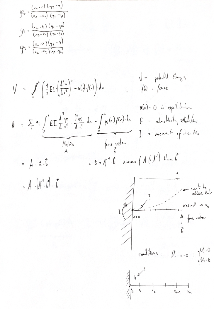
c) Now find the matrix coefficients for Hermite polynomial interpolation basis functions, once again unsing elements with fixed size of h.

from sympy import *
import numpy as np
import matplotlib.pyplot as plt
%matplotlib inline

x, h = symbols('x h')

M = Matrix([
    [1, 0, 0, 0],
    [0, 1, 0, 0],
    [1, h, h**2, h**3],
    [0, 1, 2*h, 3*h**2]
    ])
M

$\displaystyle \left[\begin{matrix}1 & 0 & 0 & 0\\0 & 1 & 0 & 0\\1 & h & h^{2} & h^{3}\\0 & 1 & 2 h & 3 h^{2}\end{matrix}\right]$

# Example from Fig. 9.2 
u0 = Matrix([[1], [0], [0], [0]])
u1 = Matrix([[0], [1], [0], [0]])
u2 = Matrix([[0], [0], [1], [0]])
u3 = Matrix([[0], [0], [0], [1]])

# Matrix inversion test
a0 = M.inv()*u0
a1 = M.inv()*u1
a2 = M.inv()*u2
a3 = M.inv()*u3
M.inv()

$\displaystyle \left[\begin{matrix}1 & 0 & 0 & 0\\0 & 1 & 0 & 0\\- \frac{3}{h^{2}} & - \frac{2}{h} & \frac{3}{h^{2}} & - \frac{1}{h}\\\frac{2}{h^{3}} & \frac{1}{h^{2}} & - \frac{2}{h^{3}} & \frac{1}{h^{2}}\end{matrix}\right]$

Problem 9.2

Model the bending of a beam (equation 9.29) under an applied load. Use Hermite polynomial interpolation, and boundary conditions fixing the displacement and slope at one end.

V, E, I, u, a, b = symbols('V E I u a b')
E=1 #elasticity modulus
I=1 #moment of interia
# u= ???
# f= ???
 

# rough structure - 
# haven't found how to represent equation for potential energy yet
#V=integrate(1/2*E*I*(diff(u, x, x))**2-u*f[i], ???)