Physics Informed Neural Networks

Posted on May 07, 2023

Continuous Time

Background

Continuous time PINNs are deceptively simple. Suppose we want to solve $dy/dt = f(y)$. We can use a deep neural network to model $y$ as a function of time. Training a neural network with gradient descent relies on being able to differentiate the output of the network with respect to its parameters, but we can also differentiate a network with respect to its inputs. The key idea of PINNs is just to compare this derivative with the function $f$ from the governing equation.

Specifically, by differentiating the network's output with respect to its input, we get the network's estimate of $dy/dt$. But we also have its estimate of $y$ (i.e. its regular output). So we just run this through $f$, and compare the result with the previous estimate of $dy/dt$. We can use the mean squared error of $f(y) - dy/dt$ as our objective function, evaluated at many random samples within the region of integration.

Pendulum on a Horizontally Constrained Cart

For instance, say we have a pendulum on a (horizontal) cart described by the following equations. (For a derivation of these equations, see here. Note that we don't include the external force or damping terms here.)

We can construct a neural network that takes a single input, $t$, and produces an output state vector $(x(t), v(t), \theta(t), \omega(t))$. (We could also just predict $x(t)$ and $\theta(t)$, but I'll assume we're predicting the whole state vector since it will make the explanation below a little simpler.) We shouldn't need anything too deep; for the studies below, I use three hidden layers of 128 neurons with $\tanh$ activations. I initialize the parameters using Xavier initialization (biases all zero, weights normally distributed with zero mean and standard deviation $1/\sqrt{n}$, where $n$ is the number of inputs of that layer).

We will fix our initial conditions: $(x(0), v(0), \theta(0), \omega(0))$. This also fixes the initial derivatives, based on equation 1. To encourage our network to respect these initial conditions, we will include the mean squared error between the desired initial state (and derivatives) and the predicted initial state (and derivatives) as a term in our loss function.

After $t = 0$, we need the network to respect the ODEs. To do this, we will choose many samples $t_0, \ldots, t_n$ over the range we'd like to integrate. At each $t_i$, we get the model's predicted state $(x(t_i), v(t_i), \theta(t_i), \omega(t_i))$. We can plug these values into equation 1 to compute what the derivatives should be at this point in time. But we can also differentiate our network with respect to $t$, to evaluate what the model thinks the derivatives are at $t_i$. We will include the mean squared error between the expected and predicted derivatives, averaged over all $t_i$, as the second term in our loss function. The original paper recommends stratified sampling, but for low dimensional problems it's fine to densely choose samples from a grid. I did find that it was sometimes helpful to add random jitter to my samples in each training iteration, to prevent the network from overfitting (i.e. allowing itself to violate the ODEs between static sample points).

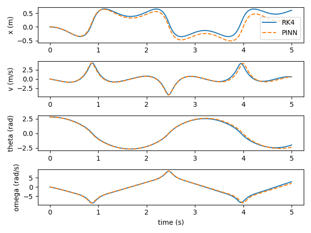
I'm training my PINN with Adam. L-BFGS seems to be more standard, but I found that it led to overfitting. The PINN performs fairly well compared to a standard RK4 integrator (with a timestep of 0.01 seconds). Here it is predicting 5 seconds of dynamics.

Pendulum on a Vertically Constrained Cart

Let's try the vertically constrained cart from the ODE assignments earlier this semester. It's pendulum is governed by the following ODE.

$$ \begin{equation} l \ddot{\theta} + (g + \ddot{z}) \sin(\theta) = 0 \end{equation} $$

We will assume sinusoidal driving of $z$: $z(t) = A \sin(\omega t)$. This reduces the ODE to the following form.

$$ \begin{equation} \ddot{\theta}(t) = \frac{1}{l} \left( A \omega^2 \sin(\omega t) - g \right) \sin(\theta) \end{equation} $$

Using equation 3, we can construct a PINN much like we did for the horizontally constrained cart. In fact the network is a little simpler, since the only state variable that we need to predict is $\theta$. As before, the network handles 5 seconds quite well.

We can also chain optimization runs together, feeding in the final state predicted by the last training round as the initial state of the next. This allows us to construct longer trajectories.

Continuous PINN Integration

The PINNs struggle to converge if we ask them to develop too long a trajectory. But we can develop a trajectory for some time $\Delta t$, then take the final state as our initial state for another round of optimization. With this gluing procedure we can develop arbitrarily long paths.

This figure shows four spliced segments, each of a one second duration. For two segments, we match RK4 quite closely. Then we diverge.

If we keep going, we're on an alternate but reasonable looking path until around 6 seconds. At this time, the network realizes that if $\theta$ and $\dot{theta}$ are both exactly zero, the ODE is satisfied forever.

In a conservative system, we could enforce conservation of energy to ensure it doesn't jump to such trivial states. For more complicated systems like this one, we would need some other additional term in our loss function.

Discrete Time

Background

Rather than use the network as a continuous function of time, we can have the network only output states for a discrete set of times. For this to work, we need some set of discrete equations derived from the governing ODEs or PDEs that relate these measurements. Luckily this is exactly what numeric integration schemes do.

I found the treatment of discrete time equations in the original paper a little hard to follow at first. Eventually I found Kollmannsberger et al's Deep Learning in Computational Mechanics, which follows the original paper very closely, but in more detail.

Runge-Kutta Methods

Suppose we want to integrate a differential equation of the form $dy/dt = f(y)$. In general, a Runge-Kutta method with $s$ stages is specified by an $n \times n$ matrix $a_{ij}$ and a vector $b_i$ of length $s$. Given these values, define $c_i$ to be the sum of the $i$th row of $a_{ij}$. To integrate forward $h$ seconds starting from $y_n$, we construct $s$ intermediate values.

$$ \begin{equation} y_{n + c_i h} = y_n + h \sum_{j = 1}^s a_{ij} f(y_{n + c_j h}) \end{equation} $$

Then we estimate $y$ in the next timestep in terms of the derivatives at these points.

$$ \begin{equation} y_{n + h} = y_n + \sum_{j = 1}^s b_j f(y_{n + c_j h}) \end{equation} $$

For explicit methods, $a_{ij} = 0$ when $j >= i$, and we can directly evaluate the intermediate values one after the other. But when $a_{ij}$ isn't diagonal, we end up with a system of equations that must be solved. For PINNs, we won't be solving the equations directly anyway, so we might as well take the increased stability that comes from implicit methods.

Runge-Kutta PINNs

To build a discrete time PINN around a Runge-Kutta scheme with $s$ stages, we construct a neural network that produces $s + 1$ values (which themselves are possibly vectors, or functions of another variable). Then we construct a loss function that encourages the first $s$ outputs to become equal to the intermediate values ($y_{n + c_i h}$), and the last output to become equal to the final value ($y_{n + h}$). We do this by constructing residuals based on equations 1 and 2.

Specifically, by running the first $s$ outputs through $f$, we obtain estimates of $f(y_{n + c_j h})$. Then we can take the mean squared values of the following expressions as our loss. To solve solve equations 1 and 2, both must be zero.

$$ \begin{equation} y_{n + c_i h} - y_n - h \sum_{j = 1}^s a_{ij} f(y_{n + c_j h}) \end{equation} $$

$$ \begin{equation} y_{n + h} - y_n - \sum_{j = 1}^s b_j f(y_{n + c_j h}) \end{equation} $$

The intermediate samples end up serving the same purpose as the random collocation points we chose in the continuous time setting. So it helps to have a lot of them. For regular numeric integration, we tend to use Runge-Kutta methods with just a few stages, as otherwise the computational cost of solving the system of equations becomes too great. But here, we just need to add another output to the network, and we're already doing gradient descent to solve the equations. So we can use several hundred stage integrators.

High Order Runge-Kutta Coefficients

The question then arises, how do you know the coefficients that determine a 100 stage Runge-Kutta method? Ultimately, Runge-Kutta methods are derived by matching terms in the Taylor expansion of the solution. John Butcher (of Butcher tableaus) has notes on how one can go about doing this. It involves summing over all "rooted trees" (particular graph structures) of degrees up to $s$.

Luckily, the authors of the original PINN paper worked out this math for us. This directory in They don't discuss it in the paper, but the GitHub repo with their code contains a directory with the coefficients for implicit Runge-Kutta integrators up to 500 stages long. They list the matrix $a_{ij}$ row by row, then $b_i$, and finally $c_i$. Here's an example of how to read them into a numpy array.

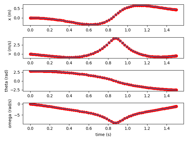
Pendulum on a Horizontally Constrained Cart

Let's use the cart-pole system again. This is using a Runge-Kutta integrator with 100 stages.