Reinforcement Learning with Policy Gradients
Posted on
Implementation
My implementation of policy gradients with rewards-to-go is here.
My objective function is a weighted sum of two terms. The first is the squared error of the pendulum angle (i.e. how far away it is from vertical in radians). The second is the square of the position of the cart (how far away it is from the origin). The second term teaches the controller to keep the pendulum in a fixed position, as otherwise it may find solutions that involve moving with constant velocity. But the angle of the pendulum is ultimately more important, so I weight the second term by 0.001. Both contributions are summed over all steps of all trajectories.
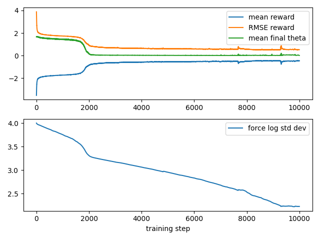
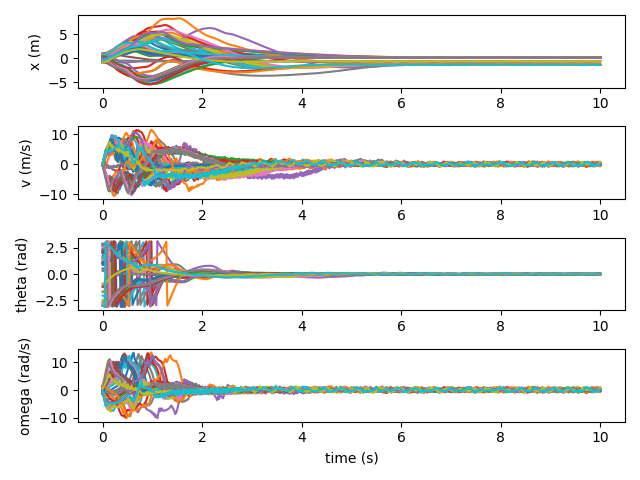
During training it tracks a variety of statistics.
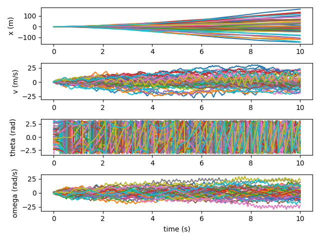
I also plot several trajectories, for a more direct view into the performance. At first, the angle of the pendulum is a complete mess, and the cart often travels quite far away.
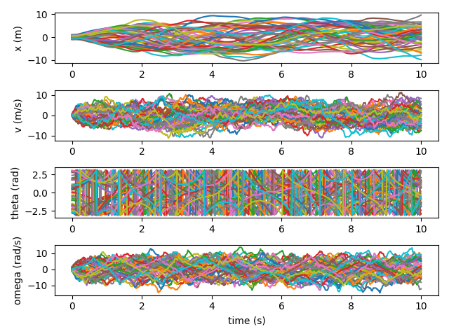
After 1000 iterations, the controller has learned how to keep the cart relatively close. And the motion of the pendulum is improving, if still quite chaotic.
After 2000 iterations, the controller has figured out how to balance the pendulum, and is learning to swing it up.
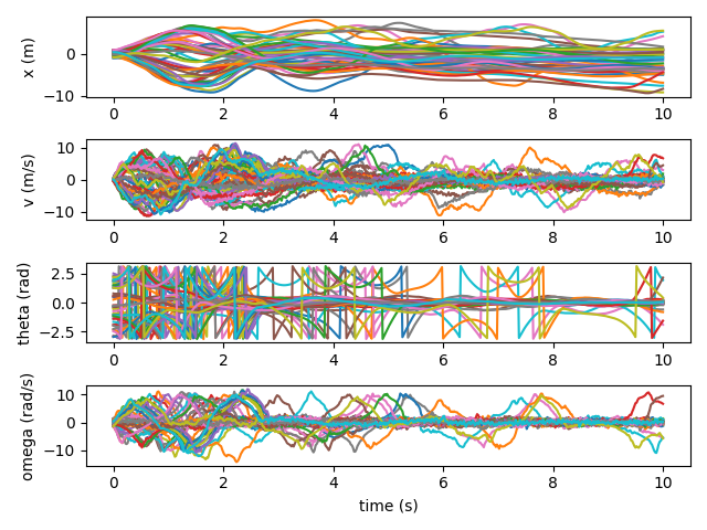
And as we approach 10000 iterations, the controller quickly swings the pendulum up and balances it nearly all the time.
I also wrote an interactive visualizer (using moderngl).
Theory
Intro
Reinforcement Learning deals with an agent acting in an environment to maximize some notion of reward over time. For example, here we'll consider the ubiquitous cartpole problem. The environment is a pendulum attached to a cart. Our agent has knowledge of the position and velocity of the cart, as well as the angular position and velocity of the pendulum, and must choose a force to exert on the cart. At each step of the simulation we give the agent a reward that measures how close the pendulum is to vertical.
There are several categories of reinforcement learning algorithms. Model free algorithms treat the environment as a black box. In practice you'll often still want a simulation of the environment so that you can more quickly collect data, but it's possible to use model free algorithms with real-world sensors and actuators even when you don't have a model. The policy gradient method explored here is a model free algorithm. Model-based algorithms require a model of the environment, often because they use it to predict the future when making decisions. For example, Monte Carlo tree search runs many randomized trials using the simulation, in order to collect statistics on which decisions lead to better outcomes.
Another broad distinction between reinforcement learning algorithms is whether they are on-policy or off-policy. The policy is the procedure the agent uses to make decisions — in particular, how the agent chooses an action which can then influence the evolution of the environment. On-policy algorithms require data collected from a particular policy in order to improve it, while off-policy algorithms can incorporate data collected via other policies.
Finally, some policies are deterministic, while others are stochastic.
Here we will consider the policy gradient algorithm, a foundational algorithm in neural reinforcement learning. It is a model free, on-policy, stochastic algorithm.
Mathematical Foundations
We will model the environment as a discrete-time Markov chain. In particular, define a trajectory to be a finite or infinite sequence of states and actions: $\tau = (s_0, a_0, s_1, a_1, \ldots)$. A policy specifies a probability distribution over actions conditional on the current state: $\pi(a_i | s_i)$. And by the Markov assumption, the distribution over possible subsequent states depends only on the current state and action: $P(s_{i+1} | s_i, a_i)$. Thus the probability of a trajectory under some policy $\pi_\theta$ factors into a product of probabilities of individual steps.
$$ P(\tau | \pi_\theta) = \left( \prod_{i=0}^N P(s_{i+1} | s_i, a_i) \pi_\theta(a_i | s_i) \right) P(s_0) $$
In the policy gradient approach, the policy is specified by a neural network. So you can think of $\theta$ in $\pi_\theta$ as the weights and biases that parametrize the network.
We will assume that rewards are determined by some function $R$ that depends on the current state, the taken action, and the next state. For each step $i$ of a trajectory, this allows us to define $r_i = R(s_i, a_i, s_{i+1})$. We will assume this function is deterministic, but the techniques discussed here can be applied to stochastic rewards as well. In particular, you can just encode the selected reward in the state, thus moving the randomness of the reward into that of the environment.
Our goal is to find a policy that maximizes some notion of cumulative reward. There are two primary axes to consider: whether the cumulative reward is computed over a finite or infinite horizon, and whether time discounting is applied. For infinite horizon rewards, time discounting is almost always applied to avoid issues with convergence.
$$\begin{aligned} R(\tau) &= \sum_{i = 0}^N r_i \quad & \text{undiscounted finite horizon reward} \\ R(\tau) &= \sum_{i = 0}^\infty \gamma^i r_i \quad & \text{discounted infinite horizon reward} \end{aligned}$$For now, we will use an undiscounted finite horizon of $N$ steps.
The reward function gives us a way to score trajectories. The policy and the environment give us a way to assess the probability of a trajectory. Thus we can evaluate policies by considering their expected cumulative rewards.
$$J(\pi_\theta) = E_{\tau \sim \pi_\theta} \left[ R(\tau) \right] = \int_\tau P(\tau | \pi_\theta) R(\tau)$$This is our key metric. Our goal is to find a policy with the highest possible expected cumulative reward.
$$ \pi^* = \argmax_{\pi_\theta} J(\pi_\theta) $$
Vanilla Policy Gradients
Recall that we will represent our policy $\pi_\theta$ as a neural network with parameters $\theta$. We'd like to have the gradient of $J$ with respect to $\theta$ in order to update our parameters. (For a more detailed derivation of the following result, see OpenAI's excellent Intro to Policy Optimization.)
$$\begin{aligned} \nabla_\theta J(\pi_\theta) &= \nabla_\theta E_{\tau \sim \pi_\theta} \left[ R(\tau) \right] \\ &= \nabla_\theta \int_\tau P(\tau | \pi_\theta) R(\tau) \\ &= \int_\tau \nabla_\theta P(\tau | \pi_\theta) R(\tau) \\ &= \int_\tau P(\tau | \pi_\theta) \left( \nabla_\theta \log P(\tau | \pi_\theta) \right) R(\tau) \\ &= E_{\tau \sim \pi_\theta} \left[ \left( \nabla_\theta \log P(\tau | \pi_\theta) \right) R(\tau) \right] \\ &= E_{\tau \sim \pi_\theta} \left[ \left( \sum_{i=0}^N \nabla_\theta \log \pi_\theta(a_i | s_i) \right) R(\tau) \right] \end{aligned}$$There are several convenient things about this result. First, we only need to differentiate our policy. We wouldn't want to differentiate through our environment since we may not have a model of our environment at all. Second, the big product in the probability calculation has been converted to a sum, which are much more numerically stable. Finally, expressing the gradient as an expectation over on-policy trajectories is convenient, because we know how to generate samples of such trajectories.
On its own, this algorithm is usually called REINFORCE or vanilla policy gradient. (Some technical distinctions can be made between these two techniques, but they are close enough that we won't worry about this now.) It can certainly solve the cartpole problem, both to keep a pendulum balanced but also to swing it up from any initial conditions.
Many algorithms extend vanilla policy gradient. The name of the game is always to reduce the variance of the policy gradient estimator. Some tricks come for free, since the reduce variance without introducing bias. Others introduce a moderate amount of bias in order to reduce the variance even further.
Rewards-to-Go
Let's take a closer look at the gradient.
$$\begin{aligned} \nabla_\theta J(\pi_\theta) &= E_{\tau \sim \pi_\theta} \left[ \left( \sum_{i=0}^N \nabla_\theta \log \pi_\theta(a_i | s_i) \right) R(\tau) \right] \\ &= E_{\tau \sim \pi_\theta} \left[ \left( \sum_{i=0}^N \nabla_\theta \log \pi_\theta(a_i | s_i) \right) \left( \sum_{j = 0}^N R(s_j, a_j, s_{j+1}) \right) \right] \\ &= \sum_{i=0}^N \sum_{j=0}^N E_{\tau \sim \pi_\theta} \left[ R(s_j, a_j, s_{j+1}) \nabla_\theta \log \pi_\theta(a_i | s_i) \right] \\ \end{aligned}$$We will show that all the terms with $j < i$ are zero.
First, let's prove a helpful lemma: the expecation of the grad log prob for any probability distribution is zero. This is called the grad log prob lemma.
$$\begin{aligned} 1 &= \int P(x) \\ 0 &= \nabla \int P(x) \\ &= \int \nabla P(x) \\ &= \int P(x) \nabla \log P(x) \\ &= E_{x \sim P} \left[ \nabla \log P(x) \right] \end{aligned}$$For any term in the double sum above, we can simplify the form of the expectation by marginalizing over irrelevant steps in the trajectory. (We may not have a good way of computing this marginal distribution, but we won't actually need to in the end.) And we can always break up expectations into conditional chains.
$$\begin{aligned} &E_{\tau \sim \pi _\theta} \left[ R(s_j, a_j, s_{j+1}) \nabla_\theta \log \pi_\theta(a_i | s_i) \right] \\ &= E_{s_i, a_i, s_j, a_j, s_{j+1}} \left[ R(s_j, a_j, s_{j+1}) \nabla_\theta \log \pi_\theta(a_i | s_i) \right] \\ &= E_{s_j, a_j, s_{j+1}} \left[ R(s_j, a_j, s_{j+1}) E_{s_i, a_i} \left[ \nabla_\theta \log \pi_\theta(a_i | s_i) | s_j, a_j, s_{j+1} \right] \right] \\ &= E_{s_j, a_j, s_{j+1}} \left[ R(s_j, a_j, s_{j+1}) \int_{s_i, a_i} P(s_i, a_i | s_j, a_j, s_{j+1}) \nabla_\theta \log \pi_\theta(a_i | s_i) \right] \end{aligned}$$When $j < i$, we can use the Markov property to simplify the conditional probability. To be completely unambiguous: from here on out we're assuming $j < i$.
$$\begin{aligned} &E_{s_j, a_j, s_{j+1}} \left[ R(s_j, a_j, s_{j+1}) \int_{s_i, a_i} P(s_i, a_i | s_j, a_j, s_{j+1}) \nabla_\theta \log \pi_\theta(a_i | s_i) \right] \\ &= E_{s_j, a_j, s_{j+1}} \left[ R(s_j, a_j, s_{j+1}) \int_{s_i, a_i} \pi_\theta(a_i | s_i) P(s_i | s_{j+1}) \nabla_\theta \log \pi_\theta(a_i | s_i) \right] \\ &= E_{s_j, a_j, s_{j+1}} \left[ R(s_j, a_j, s_{j+1}) \int_{s_i} P(s_i | s_{j+1}) \int_{a_i} \pi_\theta(a_i | s_i) \nabla_\theta \log \pi_\theta(a_i | s_i) \right] \\ &= E_{s_j, a_j, s_{j+1}} \left[ R(s_j, a_j, s_{j+1}) \int_{s_i} P(s_i | s_{j+1}) E_{a_i \sim \pi_\theta(\cdot | s_i)} \left[ \nabla_\theta \log \pi_\theta(a_i | s_i) \right] \right] \\ &= 0 \end{aligned}$$The last step follows from the expected grad log prob lemma.
This result justifies removing all terms where $j < i$ in our sum.
$$\begin{aligned} \nabla_\theta J(\pi_\theta) &= \sum_{i=0}^N \sum_{j=i}^N E_{\tau \sim \pi_\theta} \left[ R(s_j, a_j, s_{j+1}) \nabla_\theta \log \pi_\theta(a_i | s_i) \right] \\ &= E_{\tau \sim \pi_\theta} \left[ \sum_{i=0}^N \nabla_\theta \log \pi_\theta(a_i | s_i) \left( \sum_{j=i}^N R(s_j, a_j, s_{j+1}) \right) \right] \\ \end{aligned}$$If we define the reward-to-go
$$\hat{R}_i = \sum_{j=i}^N R(s_j, a_j, s_{j+1})$$we can express this more simply.
$$\begin{aligned} \nabla_\theta J(\pi_\theta) &= E_{\tau \sim \pi_\theta} \left[ \sum_{i=0}^N \hat{R}_i \nabla_\theta \log \pi_\theta(a_i | s_i) \right] \\ \end{aligned}$$Removing all the terms with expectation zero is valuable since they don't alter the mean of our gradient estimate, but they do contribute variance. Intuitively, the decisions made at any point in time can't impact the past. So it's not helpful to penalize the policy for low rewards that already happened, or give it credit it for high rewards that have already been received.