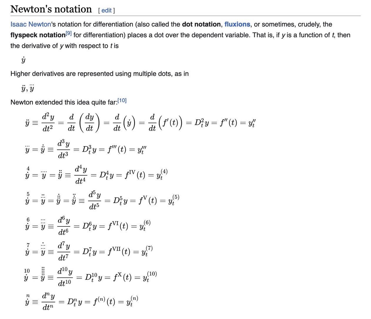
Success! The next step is to quickly decipher the notations with this Wikipedia page on Derivatives in Newton’s notation, because I had never seen Newton’s notation for differentiation before.
I started this week by documenting my work in a Google doc, including the formatting of mathematical formulas. Then I figured it's better to learn how to create mathematical equations in Jupyter. To start, this Medium article informed how to do this with Markdown. In addition, Jupyterbook provides documentation with a few examples. Jupyter uses MathJax for mathematical equations, which works with TeX/LaTex. Here is a list with commands and a quick LaTex syntax guide I found helpful. Lastly, a list with mathematical symbols. With the basics covered, let's get started!
m ̈x + γ ̇x + kx = eiωt . (4.58)
Let's first try to write this properly in JupyterLab. Using MathJax and LaTex, the same equation looks like this:
$$
  m\ddot{x}+y\dot{x}+kx=e^{i\omega t}
$$
In Markdown, this will correctly output the desired mathematical function:
Success! The next step is to quickly decipher the notations with this Wikipedia page on Derivatives in Newton’s notation, because I had never seen Newton’s notation for differentiation before.
Let’s break this down. To my understanding, small displacements of a particle around an arbitrary 1D potential minimum are very tiny changes in dx/dy (or dx/dt) at a local minimum of a function plotted on two axes. The source is a 3Blue1Brown video, Differential equations, a tourist's guide. Additionally, I watched their full series on the essence of calculus and the essence of linear algebra because I lack education in those areas. (thanks for the recommendation, Jack!)
The simplest step-by-step resource on calculating waves and oscillations I could find is this article by David Morin. Chapter 1.1 goes into simple undamped harmonic motion, and provides equations for it:
The author mentions that ‘the best tool for seeing what a function looks like in the vicinity of a given point is the Taylor series, so let’s expand V(x) in a Taylor series around $x_0$ (the location of the minimum)’. Here is another 3Blue1Brown video tutorial on what a Taylor series is and how to calculate it. In my own words, it is a method to approximate the trajectory of the curve at a certain domain using simple polynomial functions.
We start with:
$$ F=ma $$$$ F=m\frac{d^2x}{dt^2} $$$$ F=m\ddot{x} $$$$ m\ddot{x}=-kx $$Then do a Taylor at 0: $$ V=V0+V'1+V'' $$
It is a homogeneous equation, if ‘every term involves either the unknown function or its derivatives’ (NMM, p.9). You get two results: real and imaginary.
Learing from the Wikipedia page of a Damped harmonic oscillator:
$\omega$ is called the "undamped angular frequency of the oscillator"
$ζ = \frac{c}{2 \sqrt{m k}}$ is called the "damping ratio".
The value of the damping ratio ζ critically determines the behavior of the system. A damped harmonic oscillator can be:
How does the amplitude depend on the frequency? Not at all.
It is an inhomogeneous equation when there is a term that depends on the independent variable alone (i.e. a forcing term). (NNM, p.9). Real part solves imaginary part, imaginary part solves the real part.
This is what I know about springs in structural engineering. The spring constant k is dependent on material properties and dimensions of the structure:
$$ k_{eq}=\frac{EA}{L} $$Where E = Young's modulus, A = cross-secional area of the bar, and L = length of the bar before loading. But we're going to forget that for this assignment, because our goal is to approximate the curve, not to solve it with an exact answer.
Below are screenshots from my Google doc. Let's start with an ansatz.
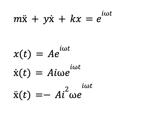
Next, plugging this in:
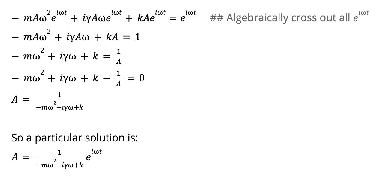
The solution written again in LaTex:
$$ A=\frac{1}{-m\omega ^2+i \gamma \omega +k} $$A is the amplitude.
Here are the numbers: $$ m = k = 1, γ = 0.1 $$
From David Morin's paper, we know that the (angular) frequency of the motion in a Hooke’s-law potential is:
$$ \omega = \sqrt{\frac{k}{m}} $$That means the following in this example: $$ \omega = \sqrt{\frac{1}{1}} $$ $$ \omega = 1 $$
The next step is to plot the function. To quickly prototype and experiment with mathematical functions, I used this free, online tool. Here is a guide on integrating this in Jupyter.
Next up: plotting with Python. In class, it was recommended to do this with Python & SciPy & matplotlib. This Medium article helps in getting a better understanding of how to do this. For this task, I'm going to try working with NumPy (Numerical Python) and matplotlib visualization for Python. Both have extensive documentation. Matplotlib offers a quickstart guide and a couple of helpful cheatsheets to get started.
import numpy as np
import matplotlib.pyplot as plt


X = np.linspace(0, 4*np.pi, 1000) # This creates a line at (start, stop, number of samples to generate)
Y = np.sin(X) # Adding a sinus function of X


plt.plot(X, Y)
plt.ylabel("Position")
plt.xlabel("Time")
plt.title("Oscillator experiment", fontsize = 14)

plt.show()

Next, let's plot the assignment.
import numpy as np
import matplotlib.pyplot as plt

k = 1
m = 1
gamma = 0.1

omega = np.linspace(0, 2) # Draw a line from x=0 to x=2

A = 1 / (-m * omega * omega + 1j * gamma * omega + k) # Formula with complex number j instead of i


A_magnitude = np.abs(A) # In absolute values (https://numpy.org/doc/stable/reference/generated/numpy.absolute.html)
A_phase = np.angle(A) # In angles (https://numpy.org/doc/stable/reference/generated/numpy.angle.html)


plt.figure()
plt.plot(omega, A_magnitude)
plt.ylabel("Position")
plt.xlabel("Frequency $\omega$")


plt.plot(omega, A_phase)
plt.ylabel("Position")
plt.xlabel("Frequency $\omega$")
plt.title('Damped Harmonic Oscillator', fontsize = 16)


plt.show()

That's a first! Let's explore the possiblities for making the plot look a little nicer.
import numpy as np
import matplotlib.pyplot as plt

k = 1
m = 1
gamma = 0.1

omega = np.linspace(0, 2, 1000) # Increasing step resolution for a smoother curve

A = 1 / (-m * omega * omega + 1j * gamma * omega + k) # Formula with complex number j instead of i


A_magnitude = np.abs(A) # In absolute values (https://numpy.org/doc/stable/reference/generated/numpy.absolute.html)
A_phase = np.angle(A) # In angles (https://numpy.org/doc/stable/reference/generated/numpy.angle.html)


plt.figure()
plt.plot(omega, A_magnitude, color="purple", label="magnitude")  # Adding color and label
plt.xlabel("Frequency $\omega$")

plt.plot(omega, A_phase, color="pink", label="phase") # Adding color and label
plt.title('Damped Harmonic Oscillator', fontsize = 14)

plt.legend() # Adding a legend
plt.text(1.5,1.75, 'magnitude') # Or annotate with inline text
plt.text(1.5,-2.25, 'phase')


plt.show()

Kinetic energy + potential energy
The potential energy stored in a simple harmonic oscillator at position x is (wikipedia):
$$ U=\frac{1}{2}kx^2 $$Kinetic energy:
$$ E=\frac{1}{2}mv^2 $$The motion of a simple harmonic oscillator is characterized by its period
$$ T = 2 \pi/\omega $$The time for a single oscillation or its frequency
$$ f = 1/T $$Kinetic energy + potential energy
The potential energy stored in a simple harmonic oscillator at position x is (wikipedia):
$$ U=\frac{1}{2}kx^2 $$The motion of a simple harmonic oscillator is characterized by its period
$$ T = 2 \pi/\omega $$The time for a single oscillation or its frequency
$$ f = 1/T $$As a reminder, the equation is:
Here's a video tutorial on how to solve a damped harmonic oscillator with Laplace transforms.
Next:
Answer
Answer
Answer