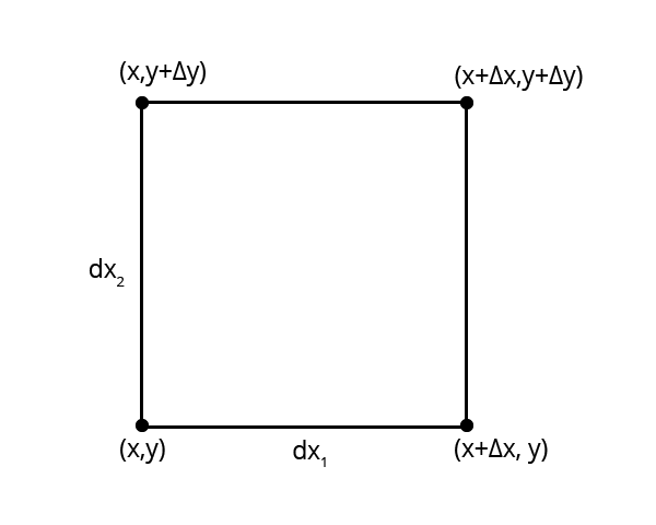
Let's start with visualizing the differential element:
Find the expected value of the transformation.
$\langle x \rangle $ = the expected value
$\bar{x}$ = vector
$\overrightarrow{X}$ = matrix vector?
n! = Factorial: Denoted by the exclamation mark (!). Factorial means to multiply by decreasing positive integers. For example, 5! = 5 ∗ 4 ∗ 3 ∗ 2 ∗ 1 = 120
Convolution = a mathematical operation on two functions (f and g) that produces a third function (f*g) that expresses how the shape of one is modified by the other. The term convolution refers to both the result function and to the process of computing it (source: wikipedia).
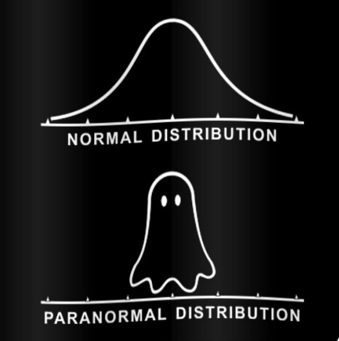
A cumulant of a probability distribution are a set of quantities that provide an alternative to the moments of the distribution. According to wikipedia, the first cumulant is the mean, the second the variance, and the third is the same as the third central moment.
Visually, this comes down to:
Some more sources in an attempt to understand cumulants:
The characteristic function:
$$ \log \langle e^{ikx} \rangle = \sum _{n=1}^{\infty} \frac{(ik)^n}{n!}C_n $$Two equations are given, with the characteristic function (7.25):
$$ exp \left(\sum _{n=1}^{\infty} \frac{(ik)^n}{n!}\right)C_n = \sum _{n=0}^{\infty} \frac{(ik)^n}{n!} \langle x^n \rangle $$and expanding the exponential as (7.26):
$$ e^x = 1 + x + \frac{x^2}{2} + \frac{x^3}{6} + \dots $$The goal is to rework the equation to find $C_n$. We do this by looking at the righthand side and lefthand side independently.
The equation on the right hand side is as follows:
$$ \sum _{n=0}^{\infty} \frac{(ik)^n}{n!} \langle x^n \rangle $$As stated above, $\langle x^n \rangle $ is the expected value. The equation goes until infinity, but we're only looking for three cumulants. Therefore, we plug in $n=0, n=1, n=2$ and $n=3$.
| n | plugged in equation | result |
|---|---|---|
| n = 0 | $$\frac{(ik)^0}{0!} \langle x^0 \rangle $$ | $$1$$ |
| n = 1 | $$\frac{(ik)^1}{1!} \langle x^1 \rangle $$ | $$ik\langle x \rangle $$ |
| n = 2 | $$\frac{(ik)^2}{2!} \langle x^2 \rangle $$ | $$\frac{-k^2}{2} \langle x^2 \rangle $$ |
| n = 3 | $$\frac{(ik)^3}{3!} \langle x^3 \rangle $$ | $$\frac{-ik^3}{6} \langle x^3 \rangle $$ |
Now let's move on to the left hand side.
$$ exp \left(\sum _{n=1}^{\infty} \frac{(ik)^n}{n!}\right)C_n $$Add m as an intermediate step to eventually remove the exponential.
$$ \sum _{m=0}^{\infty} \frac{1}{m} \left(\sum _{n=1}^{\infty} \frac{(ik)^n}{n!}C_n \right)^m $$Next, plug in the results from the right hand side.
$$ \sum _{m=0}^{\infty} \frac{1}{m!} \left( \frac{ik}{1}C_1 + \frac{-k^2}{2}C_2 + \frac{-ik^3}{6}C_3 \right)^m $$The next step is to plug in values for m.
| m | plugged in equation | result |
|---|---|---|
| m = 0 | $$1$$ | |
| m = 1 | $$\sum _{m=1}^{\infty} \frac{1}{1} \left( \frac{ik}{1}C_1 + \frac{-k^2}{2}C_2 + \frac{-ik^3}{6}C_3 \right)^1 $$ | $$ik C_1 + \frac{-k^2}{2}C_2 + \frac{-ik^3}{6}C_3 + \dots $$ |
| m = 2 | $$\sum _{m=2}^{\infty} \frac{1}{2} \left( \frac{ik}{1}C_1 + \frac{-k^2}{2}C_2 + \frac{-ik^3}{6}C_3 \right)^2 $$ | $$\frac{1}{2}\left[-k^2C_1^2 + \frac{-ik^3}{2}C_1C_2 + \dots \right]^2 $$ |
| m = 3 | $$\sum _{m=3}^{\infty} \frac{1}{6} \left( \frac{ik}{1}C_1 + \frac{-k^2}{2}C_2 + \frac{-ik^3}{6}C_3 \right)^3 $$ | $$\frac{1}{6} \left[ -ik^3C_1^3 + \dots \right]^3 $$ |
The next step is to fill in k to find the three cumulants.
We start with putting the left and right side together.
$$ikC_1 = ik \langle x \rangle $$Next, fill out k = 1
$$i1C_1 = i1 \langle x \rangle $$Resulting in:
$$C_1 = \langle x \rangle $$Thus, the first cumulant $C1$ is $\langle x \rangle$, the expected value of $x$.
For the second cumulant, the left and right hand side are:
$$ \frac{-k^2}{2}C_2 - \frac{1}{2}k^2C_1^2 = \frac{-k^2}{2}\langle x^2 \rangle $$Simply filling out k = 2
$$ \frac{-2^2}{2}C_2 - \frac{1}{2}2^2C_1^2 = \frac{-2^2}{2}\langle x^2 \rangle $$We know what $C_1$ is from the previous step, and plug this in:
$$ \frac{-C_2}{2}- \frac{\langle x \rangle ^2}{2} = -2 \langle x^2 \rangle $$Algebraically solving:
$$C_2= \langle x^2 \rangle - \langle x \rangle^2 $$Lastly, the left and right hand side of the third cumulant are:
$$ \frac{-ik^3}{6}C_3 - \frac{ik^3}{2}C_1 C_2 - \frac{-ik^3}{6}C_1^3 = \frac{-ik^3}{6}\langle x^3 \rangle $$Next, dividing everything by $ik^3/6$ gives:
$$ -C_3 -3C_1C_2 - C_1^3 = - \langle x^3 \rangle$$We know that $C_1 = \langle x \rangle$, and plug this in. Then divide everything by -1 to improve readability.
$$ C_3 + 3 \langle x \rangle C_2 + \langle x \rangle^3 = \langle x^3 \rangle$$Next, plug in $C_2= \langle x^2 \rangle - \langle x \rangle^2 $ and bring everything but $C_3$ to the right side.
$$ C_3 = \langle x^3 \rangle - \langle x \rangle^3 - 3 \langle x \rangle \left( \langle x^2 \rangle - \langle x \rangle^2 \right) $$Expanding out gets us closer to the third cumulant:
$$ C_3 = \langle x^3 \rangle - \langle x \rangle^3 - 3 \langle x \rangle \langle x^2 \rangle + 3 \langle x \rangle^3 $$The final solution for the third cumulant is:
$$ C_3 = \langle x^3 \rangle - 3 \langle x \rangle \langle x^2 \rangle + 2 \langle x \rangle^3 $$Let's start with visualizing the differential element:
Find the expected value of the transformation.
The area of the paralellogram can be calculated by multiplying the length of its base by its height.
looks like a derivative. (dy_1/dx_1)dx_1 (dy_2
Cross-product of this is the determinant
Make a diagram to visualize.
I assume that $p$ is probability.
Plugging in $y_1$ and $y_2$ gives:
$\overrightarrow{x} = \sqrt{-2 \ln x_1} \sin(x_2)(x_1, x_2), \sqrt{-2 \ln x_1} \cos(x_2)(x_1, x_2))$
Jacobian's inverse is the same as the Jacobian of the derivative (Miana):
$J_f^{-1} = J_{f'}$
Notes:
Transform by equation
Random number generator
import numpy as np

rng = np.random.default_rng(seed=42) # Input

arr2 = rng.random((3, 3)) # Place it in a 3x3 matrix

arr2 # Print results
array([[0.77395605, 0.43887844, 0.85859792],
       [0.69736803, 0.09417735, 0.97562235],
       [0.7611397 , 0.78606431, 0.12811363]])
An LFSR is a Linear Feedback Shift Register. It is a method to generate random numbers, as truly pseudo-random bits. In table 7.1 we can find the tap values $i = 1,4$ at order $M=4$. So the recursion becomes:
$$x_n=x_{n-1} + x_{n-4}$$Next, compute the values using Python, given the The recursion relation in (7.75):
$$ x_n = \sum _{i=1}^{M}a_ix_{n-i} $$With the help of a short how-to on Python random by GeeksforGeeks, a good blogpost on LFSR, a W3Schools list with Python arithmetic operators and the Python Random Module on W3Schools, here's a bit sequence:
import random

def randombit(): # Define the random number.
    return random.randint(0,1) # Return a random integer between 0 and 1.

LFSR = [randombit(), randombit(), randombit(), randombit()] # Create the register with 4 values on each line.

for i in range(len(LFSR)**2): # Adding a for loop, range() and len() function to return the number of items in an object. https://www.w3schools.com/python/python_for_loops.asp & https://www.w3schools.com/python/ref_func_len.asp
    print(LFSR)
    x = (LFSR[0] + LFSR[3]) %2
    LFSR.pop(3) # Removes the element at the specified position 3 (note: 0 is the first element). https://www.w3schools.com/python/ref_list_pop.asp
    LFSR.insert(0,x) # Inserts specified value at position x.
[1, 0, 0, 1]
[0, 1, 0, 0]
[0, 0, 1, 0]
[0, 0, 0, 1]
[1, 0, 0, 0]
[1, 1, 0, 0]
[1, 1, 1, 0]
[1, 1, 1, 1]
[0, 1, 1, 1]
[1, 0, 1, 1]
[0, 1, 0, 1]
[1, 0, 1, 0]
[1, 1, 0, 1]
[0, 1, 1, 0]
[0, 0, 1, 1]
[1, 0, 0, 1]
In the text, it is given that the repeat time is $2^n-1$ for a register with $n$ steps.
A frequency of 1 Hz is equivalent to one cycle per second. A clock rate of 1 GHz is $10^9$ Hz.
There are $60 \cdot 60 \cdot 24 = 86,400$ seconds in a day. Multiplied by 365 we have $31,536,000$ seconds in one year.
Therefore, the age of the universe is: $3.1536 \cdot 10^7 \cdot 10^{10} = 3.1536 \cdot 10^{17}$ in seconds.
In class, it was mentioned that $2^{10}$ is approximately $10^3$.
Bringing it together, and calculating the last step with Wolfram Alpha:
$$2^n - 1 = 10^{9}\cdot 3.1536 \cdot 10^{17}$$$$2^n - 1 = 3.1536 \cdot 10^{26}$$$$n = \log_2 (3.1536 \cdot 10^{26}+1)$$$$n \approx 88 $$The diffusion equation (7.57) is:
$$ \frac{\partial p}{\partial t} = \frac{\langle \delta^2 \rangle}{2 \tau} \frac{\partial^2 p}{\partial x^2} $$Resources used for answering this question include: the explanation on a Fourier transform by 3Blue1Brown, a wikipedia page on Fourier transform (not so helpful), and the textbook A First Course in Differential Equations with Applications by Dennis G. Zill.
On page 526 of the textbook, it is explained how you can do a Fourier transform. Integral transforms appear in transform pairs.
Brownian motion arises from the many impacts of the fluid molecules on the particle; let τ be a time that is long compared to these impacts, but short compared to the time for macroscopic motion of the particle (NMM book).
You want to use 24 or 32 bits (advice from Scott). Here is an example of a random walk in 3D by matplotlib.